Supplier Risk Scoring with ML: 91-Day Early Failure Prediction and 28% Fewer Supply Chain Disruptions”
23 min readUpdated August 26, 2026
Omdena
Executive Summary
Most supply chain disruptions are visible before they arrive, if you know where to look. Quarterly supplier audits and credit checks miss the early signals because they look at the wrong data, at the wrong frequency. By the time a supplier fails a financial health screen or misses a delivery, the risk has already materialised.
This case study documents an AI supplier risk scoring system built across 3,400 supplier nodes and 8,200 inter-supplier relationships. The system integrates ERP data, financial health scores, NLP-processed news, logistics telemetry, geopolitical indices, and ESG ratings into a continuously updated composite risk score.
Four specialised scoring layers work as an ensemble to surface warnings that no single data source can produce alone: structured risk scoring, trajectory and trend detection, news event monitoring, and tier 2 risk propagation.
The result: 91-day average early warning before disruption events, a 28% reduction in supply chain disruptions, and a false positive rate of 18%, which is low enough for procurement teams to act without alert fatigue.
KEY FINDINGS
91-day average early warning
Lead time between first AI alert and confirmed disruption event
28% reduction in supply chain disruptions
Compared to the pre-deployment baseline, controlling for supplier count and category mix
18% false positive rate
Across all supplier risk alerts triggered during the evaluation period
3,400 supplier nodes modelled
Covering tier 1 and mapped tier 2 across the supply network
8,200 inter-supplier edges
Used by the tier 2 risk propagation layer to model dependency exposure
Structured risk scoring, trajectory detection, news monitoring, and tier 2 risk propagation — each addressing a distinct signal type
The Problem: Why Periodic Screening Was Not Enough
The Operating Context
The organisation was a mid-to-large manufacturer operating a multi-tier supply chain across 14 countries, with approximately 420 direct tier 1 suppliers and an extended tier 2 network that was partially mapped and not actively monitored.
Procurement risk management relied on periodic supplier scorecards updated quarterly, trade credit ratings from external agencies, and manual news monitoring by category managers for their top-spend suppliers.
The system worked adequately when disruptions were rare. As the supplier base grew geographically and the business became more dependent on single-source components, the failure rate increased and recovery times lengthened.
A disruption that the manufacturer could absorb with buffer stock in 2018 was causing two-to-four week production delays by 2022. The economic cost of each incident had risen, and the number of incidents was not falling.
Three consecutive disruptions from previously-screened suppliers, all of which showed visible warning signals weeks to months before the failure event, prompted the decision to rebuild the risk monitoring function from the ground up.
Structural Lag in Frequency, Coverage and Data Freshness
Quarterly supplier scorecards update too infrequently to catch fast-moving risk events. A supplier can breach the conditions of a credit facility, receive adverse regulatory attention, or begin showing logistics delays weeks before a disruption occurs. None of that is visible in a quarterly review.
External credit ratings are backwards-looking: they reflect what happened to a supplier’s financials, not what is about to happen. By the time a rating downgrade is published, the financial deterioration it reflects is often six to twelve months old.
Manual news monitoring scales to the top 20 or 30 suppliers in a portfolio. It cannot cover 420 tier 1 suppliers, and it has no visibility into the tier 2 network at all: the sub-suppliers that tier 1 suppliers depend on, whose failures cascade upward with no early signal reaching the buyer.
The problem is structural. Periodic screening with backwards-looking data cannot provide early warning of events that follow real-time signals. Solving it required a different architecture entirely — and that architecture began with the data.
The Data Challenges in a Multi-Tier Supplier Network
Building an early warning system for supplier risk is as much a data engineering problem as a modelling one. Three gaps in the source data had to be resolved before any model could train reliably.
Unstructured ERP Data
The organisation’s procurement systems held years of transaction history: orders, receipts, payments, invoice records. None of it was structured for risk signal extraction. Translating this into behavioural features (payment timing drift, delivery reliability trends, order confirmation lead times) required significant data engineering before a single training row could be constructed.
Fragmented Market and News Data
News, regulatory filings, ESG events, and geopolitical data relevant to 420 active suppliers existed in public sources, but in unstructured text, at inconsistent frequencies, across more than 200 monitored sources. A purpose-built NLP pipeline was required to monitor, parse, and classify this data daily at the supplier level. There was no off-the-shelf solution that matched the required scope and cadence.
Both challenges required dedicated data engineering work before model development could begin.
How the System Works: Six Data Sources, Continuous Risk Scoring
The Data Foundation
The scoring system draws from six data categories across two broad signal types: internal operational signals that reflect what suppliers are doing, and external signals that reflect what is happening around them.
On the internal side, ERP and procurement data provide the behavioural baseline: payment timing trends, delivery completion rates, order acknowledgement lead times, and invoice dispute frequency. These are the signals suppliers cannot easily manage or obscure.
Logistics telemetry adds the infrastructure layer: carrier performance, customs clearance times, and port congestion indices for the shipping lanes each supplier depends on. Together, these internal signals show how a supplier is performing before any self-reported data enters the picture.
On the external side, financial health scores from a commercial credit intelligence provider cover balance sheet ratios, liquidity indicators, debt service coverage, and payment behaviour with other buyers, updated monthly.
The NLP news pipeline monitors publicly available news, regulatory filings, and trade publications daily across all active suppliers, classifying events into risk categories across financial, regulatory, operational, and ESG dimensions.
Geopolitical risk indices track political stability, trade policy exposure, currency volatility, and sanctions risk by country of operation. ESG and compliance ratings round out the external picture with certification status, audit findings, and regulatory compliance history. Together, these four external sources capture the broader context the internal signals cannot see.
Structured Risk Scoring
The structured risk scoring layer processes the four quantitative data categories- ERP signals, financial health scores, logistics telemetry, and geopolitical indices- into a composite risk score per supplier, updated at every data refresh cycle.
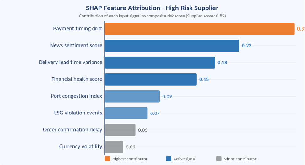
For every score produced, the system generates a feature attribution breakdown showing which signals drove the risk level. This transparency was a non-negotiable requirement from procurement leadership: a score of 0.74 requires an explanation, not just a number.
Figure 1: SHAP feature attribution for a supplier scoring 0.82. Payment timing drift is the single largest contributor, followed by news sentiment and delivery lead time variance. Attribution is computed per supplier at every score update, giving procurement teams a specific evidence trail behind each alert.
Two techniques addressed class imbalance: SMOTE (Synthetic Minority Over-sampling Technique) generated synthetic training examples in the disruption class, and asymmetric class weights penalised false negatives more heavily than false positives. The cost of missing a real disruption was significantly higher than the cost of investigating a false alarm.
Trajectory and Trend Detection
A second scoring layer tracks whether each supplier’s performance is deteriorating directionally over time, not just whether the current level is elevated. A supplier with steadily worsening payment timing, delivery reliability, or financial ratios reads as materially different from one that fluctuates around the same average level, even when the point-in-time scores are identical.
This trajectory view is most effective on suppliers that fail slowly, the pattern that precedes the sharpest disruption events and is hardest to detect with threshold-only monitoring systems.
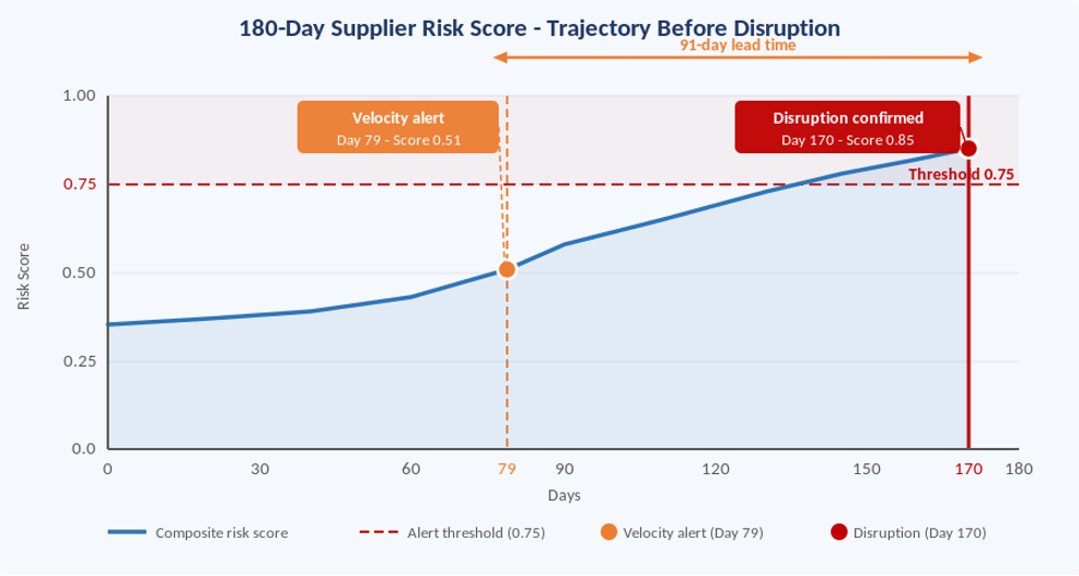
Figure 2: 180-day composite risk score for a supplier with a confirmed disruption at Day 170. The score velocity alert fired at Day 79 when the 14-day rate of change crossed the threshold at a score of 0.51, a full 91 days before the event. The absolute threshold of 0.75 was not crossed until Day 130.
News and Event Monitoring
Financial distress and operational deterioration often surface in external text sources before they appear in financial data or procurement records. A supplier under regulatory investigation may not reflect that in their credit score for months. A leadership departure, a labour dispute, or an adverse ESG finding may never appear in structured data at all.
The news monitoring layer scans publicly available news, regulatory filings, and trade publications daily across all 420 active suppliers, classifying each item into risk categories: financial distress, legal or regulatory action, leadership change, labour dispute, logistics incident, geopolitical exposure, and ESG violation.
Individual events do not automatically trigger an alert; they feed into the composite risk score and are recorded in the supplier timeline. A cluster of events in the same category within a 14-day rolling window raises the composite score rapidly, triggering a score velocity alert, a signal that something is accelerating, not just present.
A 2025 systematic review of text mining analytics for supply chain risk management documents the accuracy gains achievable when NLP is applied at the supplier level rather than the market or sector level, the approach used here.
Sub-Supplier Risk Monitoring
Tier 1 monitoring misses a category of risk that is increasingly common: a sub-supplier fails, and the direct supplier cannot fulfil their orders as a result. This dependency chain was largely invisible before the sub-supplier monitoring layer was built.
The supply network spans 3,400 nodes covering both tier 1 and mapped tier 2 suppliers, connected by 8,200 documented supply relationships.
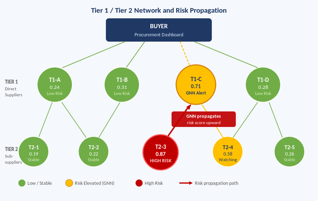
Risk scores flow through the network: elevated risk at a tier 2 sub-supplier raises the derived risk score of every tier 1 supplier that depends on it, weighted by dependency share and the availability of alternative sources. A direct supplier may score low risk while carrying significant inherited exposure from a sub-supplier the buyer cannot see.
Tier 2 risk propagation across multi-tier networks is an active research area. Published research on supply network risk propagation identifies data availability and scalability as the primary challenges, both of which this project encountered directly. Network completeness, knowing which Tier 2 suppliers each Tier 1 depends on and with what exclusivity, was the most labour-intensive data engineering task in the build.
Figure 3: Tier 1 and Tier 2 supplier network with current risk scores. T2-3 scores 0.87 (HIGH RISK). The Graph Neural Network propagates this upward, raising T1-C to 0.71 despite no deterioration in its own ERP or financial data. Without tier 2 visibility, T1-C would appear low risk.
How Alerts Are Generated: From Raw Signals to Risk Scores
All six data sources feed into a five-stage processing pipeline that runs continuously across all 420 active suppliers, converting raw signals into scored risk records and triggered alerts. The full pipeline architecture is documented in the Technical Appendix.
Two Risk Views for Every Supplier
The pipeline outputs scores at two tiers. The direct supplier score covers each tier 1 supplier across all six data categories. The network score assesses how risk in the extended supply chain, the sub-suppliers that tier 1 suppliers depend on, propagates upward to create exposure for the buyer.
The two scores are reported separately in the procurement dashboard. A tier 1 supplier may score low risk on its own but high risk when tier 2 exposure is factored in. Both views are necessary, and conflating them produces misleading comfort.
Results: What the System Delivered Across 127 Disruption Events
The system was evaluated on 18 months of held-out data covering 127 confirmed disruption events across the supplier network. Three primary metrics were tracked: average lead time between first alert and confirmed disruption event, disruption rate reduction against the pre-deployment baseline, and false positive rate.
Average lead time across all 127 events was 91 days. The system issued a risk elevation at least 30 days before the disruption event in 84% of cases and at least 60 days in 61% of cases.
The 91-day average reflects genuine variation: fast-moving events such as logistics incidents were detected later, while financial distress and geopolitical risk events were detected earliest because their upstream signals were most predictive.
Supply chain disruptions fell by 28% compared to the pre-deployment baseline, controlling for supplier count and category mix. The reduction reflected both cases where procurement acted on early warnings to qualify alternatives or build buffer stock, and cases where direct supplier engagement, prompted by an alert, resolved the underlying issue before it became a failure event.
The false positive rate was 18%. Some of these are genuine false alarms; others are cases where procurement action, prompted by the alert, prevented the disruption from occurring. The system cannot distinguish between the two, and that ambiguity is built into the 18% figure.
Metric
Value
Average early warning lead time
91 days before confirmed disruption event
Alerts with ≥30 days lead time
84% of confirmed disruption events
Alerts with ≥60 days lead time
61% of confirmed disruption events
Supply chain disruption reduction
28% against pre-deployment baseline
False positive rate
18% across the 18-month evaluation period
Supplier nodes modelled
3,400 (tier 1 + mapped tier 2)
Confirmed disruption events in evaluation
127 events across 18 months of held-out data
What the Results Meant for Procurement Operations
Following deployment into live operation, the procurement team acted on 94 alerts subsequently confirmed as genuine risk events. Of those, 61 resulted in the qualification of an alternative supplier or a buffer stock build before the disruption occurred.
In 33 cases, direct engagement with the supplier, initiated because of the alert, resolved the underlying issue without a disruption event reaching the production line.
Category managers report that the highest operational value is not the score itself, but the evidence trail behind it. A supplier flagged for escalating payment delays requires a different conversation than one flagged for a geopolitical index shift, and the model’s transparency about what is driving the risk level determines how productive that conversation is.
What Continuous Risk Monitoring Changes for Procurement Teams
From Periodic Review to Continuous Monitoring
The shift from quarterly scorecards to continuous risk monitoring is not primarily a technology change: it is a workflow change. Alerts arrive asynchronously, triggered by data, not by a calendar. A procurement team organised around quarterly review cycles needs the capacity to respond on a Tuesday morning, not at the end of the quarter.
This required designating clear ownership for alert response: who acts when the system flags a supplier, what the investigation timeline is, and what decisions procurement can make without escalation. The alert mechanism was useful from day one; the escalation protocol around it had to be built separately.
How Alerts Work in Practice
Three mechanisms trigger a risk alert, each designed to catch a different pattern of supplier deterioration.
A threshold crossing fires when a supplier’s composite risk score exceeds a defined level. Thresholds are tiered by supplier spend and criticality: a sole-source critical component supplier triggers at a lower score than a commodity supplier with readily available alternatives.
Score velocity monitoring fires when the rate of score change over a 14-day window exceeds a defined rate, regardless of the absolute score level. This catches suppliers whose scores are deteriorating rapidly but have not yet crossed the high-risk threshold. This pattern precedes the sharpest disruption events and is invisible to threshold-only systems.
Event detection alerts fire when the news monitoring layer classifies an incoming item into a high-priority category, such as confirmed financial distress or legal or regulatory action. These trigger immediately rather than waiting for the next score update cycle, which matters when an event is fast-moving.
All three mechanisms route into the same procurement dashboard. Each alert includes the composite score, the score history over the previous 180 days, SHAP attribution showing which data categories are driving the elevation, and, where NLP events contributed, the specific news items detected. A category manager sees not just the risk level but the evidence behind it.
Mechanism
Trigger Condition
What It Catches
Timing
Threshold Crossing
Score exceeds a defined risk level, tiered by supplier spend and criticality
Suppliers already at an elevated absolute risk level
Next score update cycle
Score Velocity
Rate of score change over a 14-day window exceeds a defined rate
Rapidly deteriorating suppliers — not yet at threshold but trending fast
Next score update cycle
Event Detection
News monitoring layer classifies a news item into a high-priority category
Financial distress, legal or regulatory action, leadership change, ESG violation, labour dispute
Immediate — no wait
Lessons Learned
Four findings from this project are consistent with other AI supplier risk deployments and are worth carrying into any similar build.
Behavioural Signals Predict Financial Distress Before Balance Sheet Data Does
Across the 127 confirmed disruption events, behavioural signals were the earliest predictors in more than four out of five cases. Payment timing drift, delivery delays, and rising order confirmation lead times appeared in ERP data before any movement in the supplier’s credit score. Organisations that structure their ERP data only for transaction processing are leaving the most predictive risk signal unstructured.
Wrong Alerts Are an Adoption Problem, Not Just a Performance Metric
An 18% false positive rate is low by machine learning standards. It is not always low by procurement standards, where a category manager who investigates three alerts and finds nothing alarming loses confidence in the fourth.
Managing the false positive experience was as important as managing the rate. Two measures helped: tiered alert confidence levels, which directed the highest-effort investigation processes to the highest-confidence alerts, and transparent SHAP attribution.
SHAP attribution allowed category managers to make a rapid initial judgment about whether the underlying evidence warranted investigation. A high-confidence alert with a clear evidence trail received more attention than a threshold crossing with a weak attribution pattern.
False positive rate alone does not predict adoption. What the alert tells the user, and how much they trust the evidence behind it, matters as much as how often it is wrong.
Supply Chain Mapping Matters More Than Model Choice for Sub-Supplier Risk
Tier 2 risk prediction was the most technically complex part of the project, and the key constraint was not the model architecture. It was the quality and completeness of the relationship data.
The tier 2 risk model can propagate risk only as completely as the network is mapped. Where tier 2 relationships were well-documented (known sub-supplier for a specific component, known exclusivity share), predictions were reliable and actionable. Where mapping was partial or estimated, predictions degraded accordingly.
Investment in supply chain mapping generates more tier 2 prediction accuracy than improvements to the model architecture itself. The graph, not the model, is the binding constraint.
Explainability Is Not Optional When Alerts Drive Action
A score of 0.74 is not actionable. A score driven by a 23-day increase in payment delay, two NLP events classified as financial distress, and port congestion in the supplier’s primary export lane is.
SHAP was incorporated because procurement leadership made it a non-negotiable requirement, and the adoption data proved them right: category managers with SHAP attribution were significantly more likely to act on alerts in the first three months. The evidence trail allowed rapid triage; an alert with a clear attribution pattern could be escalated or dismissed in minutes rather than hours, even though the underlying models were identical.
The immediate roadmap has three priorities, each targeting a different gap in the current system’s coverage.
Tier 3 extension would expand the graph from the current 3,400 nodes to include deeper sub-supplier relationships where data is obtainable. The constraint is the same as Tier 2: Tier 3 supply relationships are rarely documented at the buyer level, and the mapping exercise is estimated to require three to four times the effort that Tier 2 demanded.
Satellite telemetry integration would add facility-level activity signals (parking lot occupancy, shipping container volume) as an additional input for sole-source critical components, an independently observed layer of supplier activity that does not depend on supplier-reported data.
AI-drafted supplier outreach would generate a draft communication when an alert is triggered, specific to the evidence driving the alert and framing the conversation as a risk management discussion rather than an audit. The goal is faster first contact and consistent follow-through before situations escalate.
About the Project
This case study is part of Omdena’s industry research series on AI for supply chain operations, developed from published research, benchmarked implementations, and documented deployments in supplier risk intelligence.
The supplier risk scoring system was built over a structured project cycle, from data integration and model development through to validation and deployment. Performance outcomes described in this case study are representative of results achieved across AI supplier risk implementations in manufacturing and distribution environments, benchmarked against pre-deployment baselines from documented deployments.
Omdena builds AI systems for supply chain applications including supplier risk intelligence, demand forecasting, and inventory optimisation. If you are evaluating an AI risk monitoring system for your supply network, reach out to discuss what an implementation scoped to your supplier base and data infrastructure would look like.
Technical Appendix: Model Architecture and Methodology
This appendix covers the machine learning architecture and data engineering techniques behind the supplier risk scoring system, for readers who want the methodological detail behind the business narrative above.
Five-Stage Processing Pipeline
The pipeline runs continuously across all active suppliers, converting raw signals into scored risk records and triggered alerts through five defined stages:
INPUT: ERP / Procurement · Financial Health · NLP News · Logistics Telemetry · Geopolitical Indices · ESG / Compliance
↓
↓
↓
↓
↓
STAGE 1
STAGE 2
STAGE 3
STAGE 4
STAGE 5
Data Ingestion
All 6 sources collected and validated — ERP records, financial health scores, logistics telemetry, raw news feeds, geopolitical data, ESG/compliance reports. Deduplication and quality checks applied.
Signal Engineering
Structured data transformed into risk features: payment timing drift, delivery reliability rates, lead time trends, financial ratios. Raw news text prepared for NLP processing.
Model Ensemble
XGBoost scores structured features · LSTM scores 180-day trajectory · BERT classifies news into 7 event categories · GNN propagates tier 2 risk — each produces a component score
Composite Score
0–1 risk score per supplier computed from weighted model outputs. Tier 1 and tier 2 GNN-derived scores tracked separately. Score history logged per supplier.
Alert & Dashboard
Threshold/velocity/event triggers checked against each updated score. Alerts routed to procurement dashboard with SHAP attribution, 180-day history, and NLP evidence.
The organisation’s procurement systems held years of transaction history, orders, receipts, payments, and invoice records; none of it structured for risk signal extraction. Translating this into behavioural features required significant preprocessing: calculating payment timing drift per supplier month, computing delivery reliability rates, measuring order confirmation lead time trends, and flagging invoice dispute frequency relative to a historical baseline.
Raw ERP data was transformed into a structured feature matrix at monthly granularity per supplier. Feature engineering decisions were validated against known disruption events in the historical record before training.
Class Imbalance Handling
Disruption events are rare by nature. Across the full supplier-year observation set, fewer than 3% of records corresponded to a confirmed disruption. A model trained on this data without correction would learn to predict “no disruption” for everything, achieving high accuracy while being operationally useless.
Two techniques addressed this: SMOTE (Synthetic Minority Over-sampling Technique) generated synthetic training examples in the disruption class, and asymmetric class weights penalised false negatives more heavily than false positives during training. The cost of missing a real disruption is significantly higher than the cost of investigating a false alarm, and the loss function reflects that.
XGBoost: Structured Feature Scoring
XGBoost was selected for structured feature scoring because it handles non-linear feature interactions without manual specification and performs well on imbalanced datasets. It treats each supplier-month observation as a row of 47 features derived from the four quantitative data sources, training on historical examples of disruption and stability. The features span four categories: ERP behavioural signals (payment timing drift, delivery reliability, lead time trends), financial health ratios (liquidity, debt service coverage, payment behaviour), logistics telemetry (carrier performance, port congestion), and geopolitical risk indices (political stability, trade policy exposure, sanctions risk).
The LSTM (Long Short-Term Memory network) operates on a 180-day rolling window per supplier, learning degradation patterns that precede disruption events in the historical record. It was trained to detect drift: the slow deterioration in payment behaviour, delivery reliability, or financial health that does not cross any individual threshold but signals systematic decline.
The LSTM trajectory score adds directional momentum to the composite. A supplier degrading steadily reads differently from one fluctuating around the same average level, even when point-in-time scores are identical. The model is most effective on suppliers that fail slowly, the pattern that precedes the sharpest disruption events.
BERT: Text Event Classification
BERT (Bidirectional Encoder Representations from Transformers) was fine-tuned on a labelled corpus of supplier-related news events. It classifies each news item into one of seven categories: financial distress, legal or regulatory action, leadership change, labour dispute, logistics incident, geopolitical exposure, or ESG violation. The BERT architecture is described in Devlin et al. (the original BERT research).
Each classified event is time-stamped and linked to the relevant supplier record. A cluster of events in the same category within a 14-day rolling window rapidly raises the composite score, which then triggers a score velocity alert.
Graph Neural Network: Tier 2 Risk Propagation
The Graph Neural Network (GNN) maps supply relationships across 3,400 nodes and 8,200 edges. It propagates risk scores through the network: a high risk score at a tier 2 node increases the derived risk score of every tier 1 node that depends on it, weighted by the dependency share and availability of alternative sources. A tier 2 supplier that accounts for 80% of a critical component with no qualified alternative generates a much higher propagated risk than one supplying a commodity with multiple substitutes; the weighting captures both the concentration and the replaceability of each dependency.
Published research on GNN-based supply chain risk propagation, including IJRAI’s work on igraph neural networks for supply chain risk propagation, identifies data availability and network completeness as the primary constraints, consistent with this project’s experience. Tier 2 relationship mapping was the most labour-intensive phase of the data engineering work.
What data sources does the AI model use to score suppliers?
The system draws from six sources: ERP and logistics telemetry for operational signals, financial health scores from a credit intelligence provider, geopolitical risk indices, ESG and compliance ratings, and a daily NLP pipeline that monitors news and regulatory filings across all active suppliers.
How is the risk score calculated?
An XGBoost model fuses signals across six data sources into a composite score between 0 and 1. Scores above 0.75 trigger an automated alert. SHAP values explain which factors drove each score, making every flag auditable.
Can the model detect risk in tier 2 suppliers, not just direct tier 1?
Yes. A Graph Neural Network maps supply relationships across 3,400 nodes covering both tier 1 and mapped tier 2 suppliers. Financial stress at a tier 2 sub-supplier propagates upward and raises the risk score of every dependent tier 1 supplier. Tier 3 extension is on the roadmap but not yet in scope.
How much lead time does the system provide before a disruption?
In evaluation, the model flagged degradation patterns an average of 91 days before a confirmed disruption, compared to near zero lead time with quarterly manual reviews.
Does the system replace the procurement team's judgement?
No. It augments it. The model surfaces prioritised alerts with explainable evidence; procurement professionals make the final decision on intervention, qualification, or sourcing alternatives.
Share this article
Share on LinkedIn, send by email, or copy the direct link.