Developing an AI Assisted Collaborative Mapping Tool with Humanitarian OpenStreetMap
21 min readUpdated March 12, 2026
Basel Mousi, Arno Röder, Gijs van den Dool
1. Introduction
1.1. What is the main motive behind the project?
The Humanitarian OpenStreetMap Team (HOT) is an international team dedicated to humanitarian action and community development through open mapping by utilizing OpenStreetMap (OSM) [1].In the challenge,we have been supporting to build an open source AI-assisted mapping tool that can be used by HOT mappers to map areas for disaster resilience efficiently.
Currently, building footprints are not globally available in a consistent digital format, there are mapping initiatives like the recently released dataset from Microsoft [2], but this dataset misses out on critical locations, e.g. disaster-prone regions, like in the heavily populated area Shaheed Benazirabad, (Sindh) in Pakistan where the flooding between June to October 2022 made it difficult for aid workers to operate without accurate maps; Microsoft updated their cover recently and Pakistan has been partially included in mid-November.
OSM is a community-driven platform, and information is added to the database where users are active; this has resulted in an imbalanced dataset concentrated around populated places. The HOT tech team is building an open-source models tool (so-called fAIr [3]) that uses localized training dataset to build localized AI models that assist mappers in organized mapping campaigns. The AI assists in the footprint creation process by creating training and prediction datasets of the building footprints over a part of the region.
When the results of the finetuning process are above the set standard, the best model will be used to predict building footprints over the whole area. Instead of trying to fit the building footprints characteristics in a global mapping like other methods [2], this approach is different: the HOT methodology allows for a regional mapping, where local conditions are better represented [3].
You might ask yourself why is this useful? Why do we need to map buildings in case of a disaster?
Mapping for disaster resilience is necessary to make sense of the chaos and plan the best response to save lives, minimize suffering and reduce long-term impacts. Having an AI assisted mapping tool can help in reducing the mapping time needed to obtain the buildings’ footprints in a particular area
1.2. How is the project divided?
The project is divided into four main stages:
Preprocessing: Given a set of images corresponding to an area of interest along with their geojson labels, we need to create the rasterized data to be used by the model for training.
Model training: We need to train a semantic segmentation model on the rasterized input data.
Inference/prediction functionality: We need to provide the inference functionality for which the mapper will select an area of interest, and the model will run in sort of window fashion in 256*256 pixel windows.
Post-processing: we need to vectorize the predicted rasters.
1.3. How Is the Training Data Structured?
We are given, for 5 different regions, a small dataset that consists of aerial images from OpenAerialMap (OAM) and a geojson file that contains the polygon labels for the buildings from OSM. In order to collect such data, the mappers use a web API that was developed by HOT to select a region of interest. After they select a region of interest, the data gets downloaded along with the geojson labels on their disc. The training data will look like the data shown in figure 1.
Fig. 1: Training data of a test region. Name of aerial images containing tile information.
Where each image has is named as: SOURCE-x-y-z.png where source refers to the source of the image, mainly OAM. X and Y are the coordinates of the web map tile, which are used to calculate the coordinate values in “WGS84 / Pseudo-Mercator Projection” (EPSG:3857) [4]. The Z value refers to the zoom level of the web map tile. The labels.geojson file contains all the label polygons in WGS84 (EPSG:4326) coordinates. Creating the labels is the same process as digitizing the buildings and bringing the building footprints into OSM, with the difference that now a collection of footprints are saved with the same naming convention as the images, creating the link between polygon and image.
In the next section, we will introduce the technical background needed to understand the implementation of the project
2. Background Information
2.1. Geographic Information Systems (GIS)
Imagine yourself as a machine learning engineer that is designing a forest fire detection system. How useful would it be to build a system that detects fires without having any context about the location of the fire? You would need a location aware system to inform the users about the occurrence of a fire and the location of it. It is meaningless to know that a fire occurred without knowing where it actually is. Thus, when training your computer vision model, you will deal with geographically referenced data, and to analyze such data you would need a geographic information system. A geographic information system is a system that allows one to analyze and understand patterns in geographically referenced data [5].
2.2. Types of GIS data
GIS data can be divided into two main categories [6]:
Spatially referenced data which is represented by vector and raster formats
Attribute tables which are represented in tabular formats (eg. postal code)
Vector data is represented by points, lines, or polygons. Points have zero dimensions and are used to represent discrete data points. As they have zero dimension, we cannot use them to calculate areas or lengths. For example, points can be used to represent the location of a city or a place name. Lines are used to represent linear features like rivers and streets. As lines are one dimensional, we can use them to calculate lengths only. Finally, polygons are used to represent areas. We can use polygons to represent the location of a neighborhood. As polygons are two dimensional, we can use them to calculate areas.
In our case, the aerial images from OAM are stored in a georeferenced raster format. Raster data can be distinguished into continuous and discrete data. For example, aerial images are continuous raster, while the masks of the building footprints are discrete raster. On the other hand, the buildings from OSM are represented in a vector data format (GeoJSON). Vector data can be stored in three different data types: point, line or polygon as mentioned earlier. The buildings downloaded from OSM are polygon features.
2.3. Coordinate System and Why it Matters
As mentioned above, our input data are available in the coordinate systems WGS84 (EPSG:4326) and “WGS84 / Pseudo-Mercator Projection” (EPSG: 3857). But what is the difference between these two coordinate systems? The “World Geodetic System 1984”
(WGS84) is the most common geographic coordinate reference system which is widely used in GIS and GPS. The units of the coordinate system are degrees. The coordinates represent a point on an ellipsoid. On the other hand, the Pseudo-Mercator projection uses a Mercator projection instead of an ellipsoid. The units of the Pseudo-Mercator projection are meters. This projected coordinate reference system is widely used by web mapping applications in the Internet such as Google Maps, Bing Maps, OpenStreetMap, and OpenAerialMap. The difference between the two coordinate systems is shown in figure 2
Figure 2: Conversion process for using one projected coordinate system for both vector and raster inputThe ML-DL process is coordinate system agnostic, and works on the pixels of the images, but to geographically match the rasterized labels with the image it is important to work in the same coordinate system to get spatially congruent arrays for feeding our machine learning models. So we decided to convert the GeoJSON datasets from WGS84 to “WGS84 / Pseudo-Mercator Projection” in order to have all input datasets in a metric coordinate system. Setting the EPSG also meant that the images, stored in the OpenAerialMap database without a projection but with a TileMap Service indicator, had to be projected to the EPSG:3857 coordinate system. Usually, reprojecting images introduces a distortion, but the images are processed in EPSG:3857 before storing them in png-format with a TileMap Service identifier.
2.4. OpenAerialMap (OAM) / OpenStreetMap (OSM)
OpenStreetMap was founded in 2004 as an open data platform for editing and maintaining free geospatial data, which were contributed by volunteers. The vector datasets from OSM can be exported or downloaded in several ways. HOT provided us with GeoJSON files of the buildings for the test regions.
OpenAerialMap is an initiative maintained by HOT to manage imagery from satellites, unmanned aerial vehicles (UAVs) and other aircraft for humanitarian response and disaster preparedness. The platform was created by HOT because during and after a disastrous event (e.g. flooding, landslides, hurricanes, or armed conflicts), remote sensing data becomes increasingly available, but it is often difficult to determine what is readily available and how to access these data streams. Therefore, OAM is developed to serve as a platform for openly licensed imagery data.
2.5. Semantic Segmentation
Semantic Segmentation refers to the computer vision task of pixel-wise classification of images in which we assign a class to each pixel in the input image. This task is also referred to as dense prediction [8]. Figure 3 shows a sample expected output of a semantic segmentation model
Fig. 3: Image example for semantic segmentation
It is important to note that, unlike instance segmentation, we don’t differentiate between instances when classifying pixels. For example, in the above figure, all persons belong to the same class.
In our case, we are segmenting buildings from aerial images. Figures 4 and 5 show a black box representation of the model.
Fig. 4: Black Box representation of a segmentation modelFig. 5: Black box representation of training with aerial images and predicting building footprints
2.6. RAMP Model: A UNET with an Efficient Net Encoder
RAMP stands for Replicable AI for microplanning. It is an open-source deep learning model that accurately digitizes buildings in low- and middle-income countries (LMICs) using satellite imagery. It enables users to build their own deep learning models for their region of interest. It was trained on many different types of satellite images. It uses Eff-Unet as the deep learning model [9]. Thus, to understand the RAMP model better it is necessary to develop intuition about the UNET and EfficientNet models.
The UNET model is an encoder-decoder based CNN model that was developed for biomedical image segmentation [10]. The model contains a contracting path (the encoder) which encodes the spatial information of each image, and an expanding path (the decoder) which is able to perform precise localization using transposed convolutions. The architecture also uses symmetric skip connections between the encoder and the decoder to pass the feature map at the time at each decoding level.
The Efficient encoder network was introduced by Tan & Le (2019) [11]. Its basic building block is a mobile inverted bottleneck convolution, also called MBconv. One residual block contains an expansion layer, a depthwise layer, and a projection layer. The expansion layer increases the number of channels in the data before it goes into the depthwise convolution. We can think of it as uncompressing the input tensor. Afterward the depthwise layer makes the convolution filtering. Finally, the projection layer compresses the number of channels and so reduces the number of dimensions for the output tensor. Therefore it is also called a bottleneck layer.
Fig. 6: Bottleneck residual blockFig. 7: Concept of a bottleneck residual block [12]Fig. 8: Example for a bottleneck residual block [12]As expansion and projection are done with learnable parameters, the model learns an efficient way to decompress and compress the data. Therefore, the EfficientNet model can be scaled up very effectively, and achieves better accuracy with fewer parameters [11]. The ramp model uses an efficientnetB7 encoder which means that it uses 7 MBconv blocks.
3. Technical Implementation
3.1. Preprocessing
a. What is the main goal of this task?
The main goal of the preprocessing task is to prepare the data for training the model. We were given tile images along with a geojson file containing the corresponding polygon coordinates. We should use these images to generate the raster images needed to train the model.
It’s important to note that the tile coordinates were given in a “WGS84 / Pseudo-Mercator Projection” (EPSG: 3857)while the labels were given in WGS84 (EPSG:4326).Here’s the suggested pipeline for preprocessing:
Load the Labels (EPSG: 4326)
Reproject the labels (FROM EPSG: 4326 to EPSG: 3857)
Rasterize the labels (The labels are a mask, and they should have the same origin and dimensions are the image they are tested against)
Extract the RGB values from aerial images
Train a model on the extracted RGB values
b. What are the main steps of this task?
The preprocessing part can be separated into 3 main stages as shown in the figure below
Fig. 10: Pipeline for using a pretrained model
To dive deeper into the task, we can divide it into the following steps:
Read the tile coordinates of the image from each file name
Use these coordinates to calculate the longitude and latitude in WGS84 (EPSG:4326) [4]
Use the longitude and latitude to calculate the bounding box coordinates in “WGS84 / Pseudo-Mercator Projection” (EPSG: 3857)
Use the calculated bounding box coordinates to georeference each image with the gdal_translate command. We pass the parameter ‘a_ullr’ to override the georeferenced bounds of the image. We also pass the parameter ‘a_srs’to specify the new coordinate system (in our case we set it to EPSG:3857). We save the new images in GeoTIFF-format as the final step of the georeferencing part.
We then correct the labels by removing the self-intersections. We achieve this by using the explain_validity and make_validfrom shapely.validation
Then we clip the labels by using ogr2ogr. We specify the -clipsrc flag to indicate the coordinates of the bounding box and -f to indicate the output file format
Finally, we rasterize the clipped labels by using gdal_rasterize
c. Preprocessing using the developed Hotlib
Code example for preprocessing the input data with HOTLib
from hotlib import preprocess

preprocess(

    input_path="/content/gdrive/MyDrive/Omdena/inputs_v2",

    mask_path="/content/gdrive/MyDrive/Omdena/masks_v2",

    rasterize=True,

    image_path=None,

)
3.2. Main Training
a. What is the goal of this task?
The main goal of the task is to train a semantic segmentation model on the obtained rasters from the preprocessing stage. When training the model, one should keep in mind the following considerations.
Limited Data: We have a limited amount of data and getting more data is expensive, that’s why it is important to utilize transfer learning.
Regional diversity: A model that performs well on one region might not perform well on another as the structure of building might differ between areas. For example, a model that performs well on detecting buildings in Cairo might not perform well on detecting buildings in Nairobi.
Zoom levels: The model should be robust to buildings at different scales.
Inference time: The model should perform inference in less than 1 s for the 5*5 given region.
Model Performance: We should assess the performance of a model quantitatively and qualitatively. To assess it quantitatively, we used the intersection over union score. To assess it qualitatively, we inspected the obtained mask for randomly chosen images
To build a robust model for each of the following five regions, the team built the pipeline shown in figure 10.
Fig. 10: Pipeline for using a pretrained model
The general workflow begins by georeferencing and rasterizing the given images for a specified area of interest. We then get a pretrained model and finetune it for each region thus obtaining a separate model for each region. It is important to note that the pipeline expects to find a model that is already pretrained without having to run the training again. The team suggested to use either the open cities [13] model or the ramp model [9] for this pipeline. In case these models didn’t perform as expected for any given region, the team developed another pipeline that expects to train the model from scratch. The second pipeline is shown in figure 11.
Fig. 11: Pipeline for training a model from Scratch
b. Tested machine learning models
We tried the following models:
UNET: The team developeda UNET semantic segmentation model. The options of training the model from scratch and utilizing transfer learning were considered. For development, we used the segmentation models library that is built on top of tensorflow. We loaded the model with the pretrained weights on imagenet. For transfer learning, we used a dataset based on the open cities data [14], which is also available on Kaggle [15][16].
CNN Encoder-Decoder: The main goal was to develop a CNN encoder-decoder baseline that can be adopted for our task. The model considered the mean value of pixels across several channels which was considered as a limitation for the model
Open Cities: The goal of this task was to investigate the feasibility of adopting the open cities model for our task. The open cities model is an ensemble of UNETS that were trained on the open cities data.
Classical ML: As the data that we were given was limited, we decided to check whether we would achieve good results if we used classical ML models (namely, XGBOOST and Random Forest)
RAMP: Fine tuning the RAMP model pretrained on the large amounts of aerial imagery.
c. Model Adoption
We adopted the RAMP model as it was the best performing model for our task. The best performance of the RAMP model can be attributed to the fact that it was pretrained on large amounts of aerial imagery. Below are the obtained results for the five regions given. The fine-tuning and inference steps were done on Google Colab Pro (2 x Intel Xeon CPU 2.20 GHz, Nvidia Tesla T4 GPU).
Region 1
Region 2
Region 3
Region 4
Region 5
Batch Size
20
20
20
10
20
Number of Epochs
20
50
50
60
40
Accuracy (%)
98.7
92.3
93.5
96.6
86.6
Mean IoU (%)
92.1
83.2
81.6
88.7
72.6
Fine-tuning time
30 minutes
29 minutes
39 minutes
40 minutes
40 minutes
Inference time
2.5s
1.25s
1.5 s
1.65 s
1.7 s
The results obtained reflect the regional diversity consideration that we outlined in the previous section. Notice that the model has the highest intersection over union score for region 1 and the lowest one for region 5. The buildings in region 5 tend to be more clustered as the region represents a densely populated area while the buildings in region 1 represent a rural area where buildings are far from one another.
3.3. Inference
The goal of this task is to return the segmentation masks for a set of input images. We will be given a set of input images (in our case we considered having 5*5 images where each image is 256*256 pixels) and we will simply use the model to perform the prediction. The expected output from this task is a set of predictions for the given input images. Below is a GIF that illustrates the goal of this task.
Fig. 12: From aerial images and building masks to predicted labels
It is important to note that the given input images correspond to one region and you can stitch them back together to obtain a mosaic for this region. We were given test images for all five regions. For example, below is the mosaic of stitched images for region 1 at zoom level 20 where the predicted masks are visualized on the same mosaic.
Findings: The model performs well on region 1. The model detects the buildings accurately. In the shown example, the predicted masks are overlaid over the actual buildings
Overview
Detail
Here’s another example from region 2 using zoom level 19
Findings: The model performs well on region 2. The model detects the buildings accurately. In the shown example, the predicted masks are overlaid over the actual buildings
Overview
Detail
Does the model have any limitations?
Yes! The model fails to detect buildings in densely populated regions. Below is an example from region 5 at zoom level 20
Findings: The model does not perform well in densely populated regions. The model fails to detect the boundaries of buildings as shown in the detail figure on the left
Overview
Detail
Why do you think the model has a poor performance in such regions?
Well it can be attributed to several things. The first of which is the amount of data the RAMP model was fine tuned on. We had 541 images for region 5 only and it is suggested on the RAMP website to use 2000~4000 images for fine tuning. The second reason might be the quality of images used. Using images of higher resolution will definitely improve the performance!
3.4. Post-processing
For post-processing the inference results, our team tested several approaches. One method was the algorithm from the AutoBFE-project [17]. We implemented the building footprint extraction as polygonize function in the HOTLib library.
Code example for post-processing the inference results with HOTLib
from hotlib import polygonize

polygonize(

    input_path=f"/content/gdrive/MyDrive/Omdena/colab",

    output_path=f"/content/gdrive/MyDrive/Omdena/labels.geojson"

)
The workflow of this algorithm is as follows:
We extract the building contours of a single image tile by using OpenCV and retrieve a list of polygons.
We simplify the polygons using the Douglas-Peucker algorithm by removing all points with a distance to the straight line that is smaller than the tolerance value 0.01.
We georeference the simplified shapes to WGS84 (EPSG:4326) with the X-, Y-, Z-values from the input filenames.
We remove all self-intersections from the georeferenced shapes.
We append all polygons with a positive area to an array.
After post-processing all the resulting images, we merge the nearby polygons from the array using a buffer distance of 0.5 meter. During buffering, the border lines of the polygons are expanded and if two polygons overlap, they get merged to one.
Finally, we save the resulting list of polygons in a GeoJSON file.
4. Conclusion
In this technical case study we want to give a short introduction in the Omdena challenge “AI Assisted Collaborative Mapping Tool” and present some of the results. Based on the input data provided by the Humanitarian OpenStreetMap Team, we developed a workflow for preprocessing aerial images as well as the building footprints.
Basic knowledge in GIS and coordinate systems is necessary when working with geospatial data. We also explained the fundamentals of semantic segmentation and the RAMP model, which uses EfficientNet as encoder in an U-Net architecture. We have tested several machine learning architectures and for RAMP we received the best results after fine-tuning in terms of accuracy, IoU-score and inference time.
As a reference implementation of the workflow we developed HOTLib [18]. This python library includes post-processing functionality like the AutoBFE algorithm. Further development should be focussing on better model prediction as well as improving the automatic delineation of neighboring houses in densely built areas. These project results should enable HOT to provide their mappers with an AI assisted collaborative mapping tool for the detection of building footprints.
[11] Tan, M., Le, Q. V. (2019): EfficientNet: Rethinking Model Scaling for Convolutional Neural Networks. https://arxiv.org/pdf/1905.11946.pdf, ICML 2019.



![Figure 2: Conversion process for using one projected coordinate system for both vector and raster input (adapted from www.maptiler.com [7])](https://cmsnew.omdena.com/wp-content/uploads/2022/12/Fig-2.png)


![Fig. 6: Bottleneck residual block [12]](https://cmsnew.omdena.com/wp-content/uploads/2022/12/Fig-6.png)
![Fig. 7: Concept of a bottleneck residual block [12]](https://cmsnew.omdena.com/wp-content/uploads/2022/12/Fig-7.png)
![Fig. 8: Example for a bottleneck residual block [12]](https://cmsnew.omdena.com/wp-content/uploads/2022/12/Fig-8.png)