
AI and Drone Imagery for Real-Time Weed Detection in Precision Farming — Omdena Case Study
Explore how AI and drone imagery identify weeds in real time for precision spraying and lower herbicide costs.
May 15, 2026
22 minutes read
Executive Summary
Weeds cost arable farmers billions of dollars every year. The standard response, spraying entire fields with herbicide, works but at a high financial and environmental cost. A field in which 10% of the area is weed-infested does not need 100% chemical coverage. The precision required to spray only where weeds exist has, until recently, exceeded what was practically achievable at the farm scale.
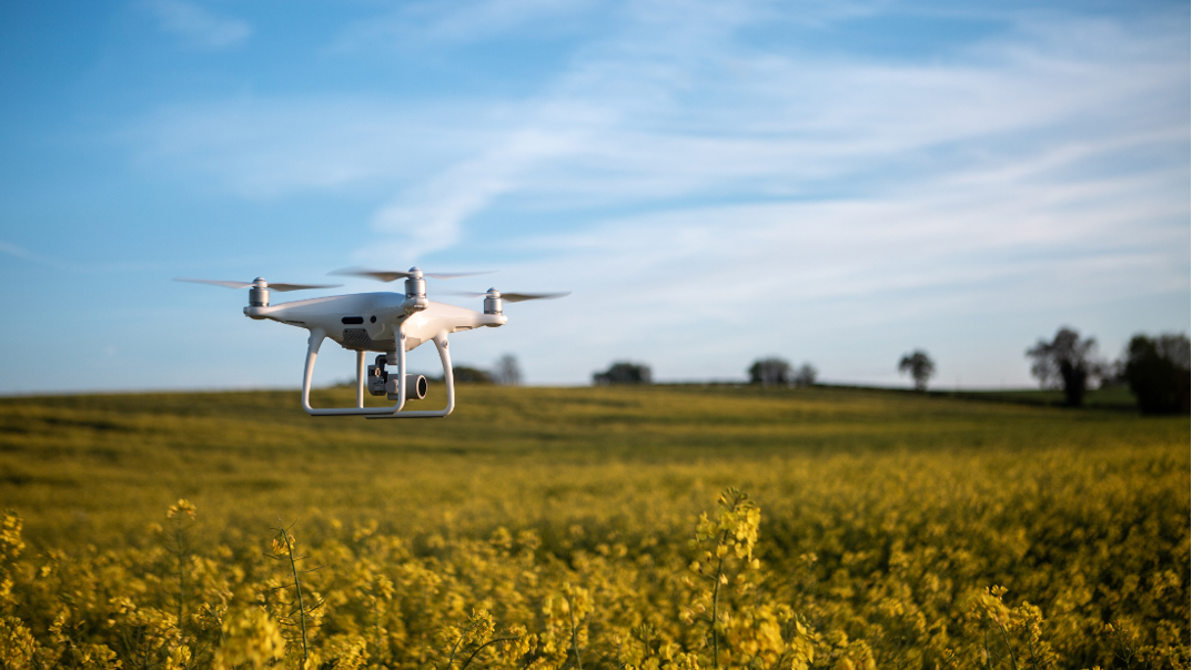
The project used drone-mounted cameras to capture centimetre-resolution aerial imagery of arable fields, then applied computer vision to locate, classify, and map every weed plant. In an 8-week Omdena collaboration, a global team of AI engineers built three complementary machine learning pipelines: an object detection system using YOLOv5 to identify and count weeds with bounding boxes, a semantic segmentation system using U-Net with EfficientNet backbone to classify every pixel as crop or weed, and a super-resolution pipeline using DCSCN to upscale lower-quality drone imagery to inference-ready resolution.
The weed detector correctly located and identified roughly two-thirds of plants in test images. Critically, a model trained on computer-generated imagery performed eight times worse than one trained on real drone photographs, confirming that real-world annotation cannot be shortcut. The pixel-mapping model reliably classified the main crop area, with weed accuracy reflecting the genuine difficulty of spotting sparse, visually variable thistle plants in real fields. The image enhancement model was the only one of the six tested to produce clean output without introducing false colours, which would have undermined the detection step.
| Key Findings |
| YOLOv5 Large: [email protected] = 0.661 · Best-performing object detector across 4 classes |
| Synthetic data penalty: [email protected] drops to 0.079 without real annotation · 8.4× gap |
| U-Net EfficientNet B0: Crop IOU ≥ 0.88 · Weed IOU 0.3–0.5 · Per-pixel field mapping |
| Mask R-CNN: Individual plant instance counting at the species level within detected zones |
| DCSCN super-resolution: Best metrics and cleanest output · GAN models disqualified by artifacts |
| Active learning (OnePanel + CVAT): Each annotation cycle improves the model and reduces future labelling cost |
Weeds, Herbicides, and the Cost of Imprecision
Every arable field contains weeds. The question is never whether they are present but where, in what density, and which species are competing most aggressively with the crop. That question matters because the economic and environmental costs of weed management are almost entirely determined by what happens next: how much herbicide is applied and where.
Broadcast spraying, the standard approach on commercial farms, applies a uniform chemical dose across the entire field. If weeds are distributed across 10% of the field area, broadcast spraying uses 10 times the amount of herbicide actually needed. The excess generates herbicide resistance in surviving weed populations, contaminates soil and waterways, increases per-hectare input costs regardless of actual infestation density, and contributes to an environmental load far in excess of what is agronomically justified.
The traditional alternative, manual field scouting, is impractical at commercial scale: a 200-hectare farm cannot be surveyed at plant-level resolution before the herbicide application window, incurring per-imaging-change costs. A UAV covers a field in minutes at two to five centimetres per pixel, making individual plants visible. Still, a single flight generates thousands of image tiles too numerous to review by hand. The only scalable path from drone capture to actionable weed maps is computer vision, which is what SkyMaps Agrimatics built in partnership with Omdena.
The Approach: Three Pipelines for Three Questions
A weed map capable of directing a variable-rate spr. Still, AEDs need to answer three questions: whether the drone imagery is sharp enough to detect individual plants at all; where in the field the weeds are located; and which pixels in each image belong to a crop plant versus a weed.
Each question corresponds to a different computer vision task, and each task requires a different model architecture. Rather than choosing a single approach, the Omdena team built all three in parallel, establishing what each pipeline delivers, where each has limitations, and how they combine into a complete system.
Super-Resolution: Making Drone Imagery Detection-Ready
The first question is a prerequisite for the other two. Not every drone flight produces imagery sharp enough for reliable weed detection — wind, sensor quality, flight altitude, and image compression all degrade it. An image enhancement pipeline takes a blurry or low-quality image as input and produces a sharper version for the detection model. Six different approaches were tested and evaluated on both technical quality scores and visual output.
Object Detection: Localising Weeds with Bounding Boxes
Object detection answers where the weeds are. Models in this category place a labelled bounding box around each detected plant, recording its location, class, and the model’s confidence in the prediction. For a drone-surveyed field, this produces a point map of weed locations that can be used directly to define spray zones. Three detectors were evaluated: YOLOv4, Faster RCNN, and YOLOv5 in its Large configuration.
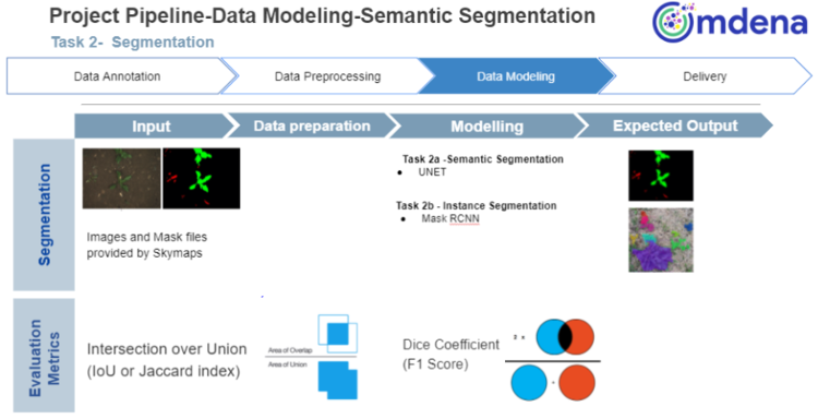
Semantic Segmentation: Classifying Every Pixel
Semantic segmentation answers which pixels belong to a crop plant and which to a weed. This provides a denser map than bounding boxes, capturing the exact shape and area of each infestation patch. The team evaluated U-Net with an EfficientNet backbone as the primary architecture and Mask R-CNN as an instance segmentation variant capable of distinguishing individual plant instances within the same class.
The Dataset: Challenges of Real Drone Imagery at Field Scale
Every computer vision project begins with data, and agricultural data presents a collection of challenges that laboratory benchmarks do not. This project encountered all of them.
SkyMaps provided aerial photographs taken by a drone at high enough resolution to distinguish individual plant leaves from above. These images were divided into smaller tiles for model training. The dataset covered four plant types: young beetroot seedlings, established beetroot rosettes, corn, and thistle weed. Treating the two beetroot growth stages separately matters for spraying decisions, since the correct response to a weed growing among small seedlings differs from that for one growing alongside taller, established plants. It also makes the visual recognition task harder, since the same crop looks quite different at each stage.
The fundamental problem with real drone agricultural imagery is visual ambiguity. Young weed seedlings photographed at canopy level look remarkably similar to young crop seedlings. Leaf overlap between adjacent plants creates partial occlusion that defeats simple template-matching approaches. Shadows cast by taller plants across shorter neighbours change local colour and texture in ways that confuse models trained without accounting for illumination variation.
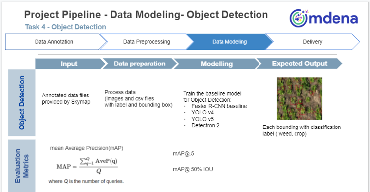
The object detection pipeline: raw drone imagery is preprocessed and tiled, passed through three detector architectures (YOLOv4, Faster R-CNN, YOLOv5), and outputs bounding-box predictions per class with confidence scores.
Two further data challenges proved central to the project. First, the class imbalance between crops and weeds in a well-managed field is severe. A field at the point of a herbicide application decision might have one weed plant for every thirty crop plants. Models trained on naively sampled data learn to predict ‘crop’ for almost every pixel and still achieve superficially high accuracy, because they are right most of the time. Detecting the rare class (the weed) requires deliberate strategies to ensure it appears frequently enough in training batches for the model to learn to recognise it.
Second, and most consequentially for this project, the team tested whether synthetically generated imagery could substitute for real annotated data. The answer was definitive: it could not.
The Synthetic Data Test: A Result That Changes the Annotation Strategy
Annotating drone imagery at the plant level is expensive. Each image tile must be reviewed by a person who can identify which green rosette is a thistle seedling and which is a beetroot cotyledon. At the resolution required for detection, a single field flight can produce tens of thousands of tiles requiring annotation. For most organisations, that cost is prohibitive.
One appealing alternative is synthetic data: generating photorealistic training images using computer graphics, with labels produced automatically by the generator. No human annotator is needed. The Omdena team tested this directly by training a YOLOv5 model on synthetically generated drone imagery of the target classes and evaluating it on real field images.
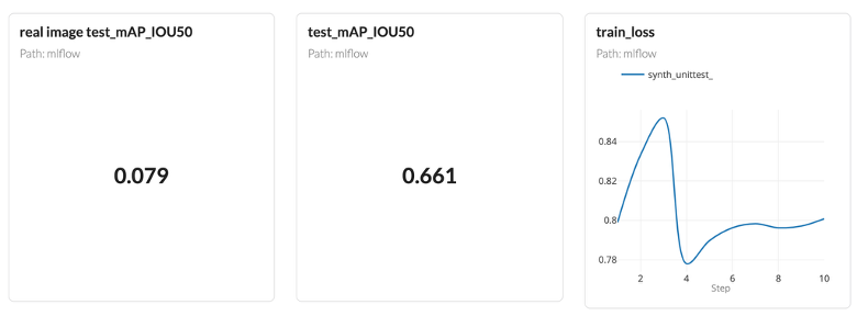
Detection performance comparison: a model trained exclusively on synthetic thistle images achieved [email protected] of 0.079 on real drone imagery (left), versus 0.661 for the same architecture trained on real annotated data (right). The 8.4x gap quantifies the domain shift penalty of synthetic-only training.
The result was unambiguous. A detector trained exclusively on synthetically generated thistle images achieved a [email protected] of 0.079 on the real field evaluation set. The same architecture, trained on real, annotated drone imagery, achieved 0.661, an 8.4-fold improvement. The synthetic images, generated by compositing cutout plant photographs onto agricultural background tiles, failed to capture the texture variation, shadow patterns, and colour noise that characterise real drone imagery captured at field scale. A model that has learned only synthetic appearances cannot reliably transfer to the visual complexity of a real field.
The implication is that real annotation is not optional for this task. The question is not whether to annotate real imagery, but how to do so efficiently. That is the problem active learning was designed to solve.
Active Learning: Scaling Annotation Without Scaling Cost
Active learning is an approach to annotation that inverts the standard workflow. Rather than labelling the entire dataset before training begins, an active learning system trains an initial model on a small labelled seed set, then uses that model to identify which unlabelled examples are most informative to annotate next.
The key insight is that not all training examples are equally valuable. A model that has already learned to distinguish beetroot from thistle at a clear viewing angle gains little from seeing another thousand well-lit, unoccluded examples. It gains a great deal from examples at the edge of its confidence: partially occluded plants, unusual lighting angles, atypical growth stages, and species combinations it has not seen before. By directing annotators to label exactly these hard cases, active learning extracts far more model improvement per annotation hour than random or sequential labelling.
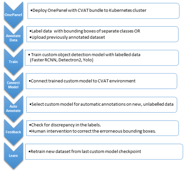
The active learning pipeline: a seed model is trained on a small labelled set, identifies low-confidence or high-uncertainty predictions on the unlabelled pool, and routes those images to CVAT for human annotation. Each cycle improves both the model and the annotation queue.
The team implemented this pipeline using OnePanel for orchestration and CVAT (Computer Vision Annotation Tool) for the annotation interface. OnePanel provides a cloud-based environment that manages the model training cycles, tracks which images have been labelled, and handles the logistics of routing uncertain images to the annotation queue. CVAT provides an annotator-facing interface for drawing labels.
An important feature of the setup is CVAT’s automatic annotation capability: models trained in each active learning cycle can be imported back into CVAT to pre-populate label suggestions for new images, which annotators then correct rather than draw from scratch. Correcting a near-correct automatic annotation takes a fraction of the time required to draw a new label from scratch, thereby substantially compressing the per-image annotation cost.
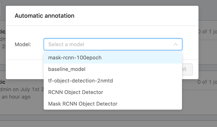
CVAT’s annotation interface with model-assisted pre-labelling. The model suggests bounding boxes and segmentation masks; the annotator corrects them. This reduces annotation time per image by 60–80% compared with manual labelling from scratch.
Over the course of the project, the active learning loop substantially improved model performance with each cycle, demonstrating that the system routed genuinely hard examples to annotators rather than generating arbitrary labelling work. The combination of active learning selection, the DAGsHub experiment, data version control, and CVAT annotation created an annotation infrastructure that could realistically scale to the volumes required for a commercial deployment.
Super-Resolution: When Drone Altitude Costs Image Quality
Every drone survey involves a trade-off between altitude and image sharpness. Flying low produces the crisp, detailed photographs the detection models need, but covering a large field at low altitude takes significantly more time. Flying higher covers more ground per pass but produces blurrier images that may fall short of the quality needed to identify individual plants reliably.
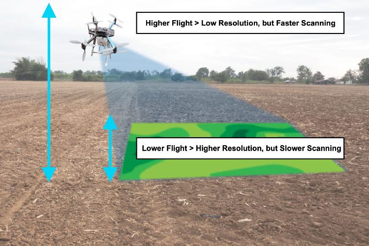
The altitude trade-off in drone field survey: a higher flight path covers more area per pass but produces lower-resolution imagery. In comparison, a lower flight path yields the sharp ground sampling distance required for plant-level detection. Super-resolution bridges this gap, allowing high-altitude survey data to reach inference-ready quality without a second low-altitude pass.
Both the detection and segmentation pipelines described in this article depend on imagery sharp enough for plant-level inference. In practice, this assumption does not always hold, and not only because of altitude. Consumer-grade drone sensors produce more compression artefacts than survey-grade equipment, and adverse flying conditions introduce motion blur. All of these reduce effective resolution, thereby degrading detection performance.
Image enhancement AI addresses this directly: a model takes a blurry or low-quality image as input and produces a sharper, higher-resolution version that the detection system can reliably work with. Six different approaches were tested and compared using standard image quality measures and visual output quality.
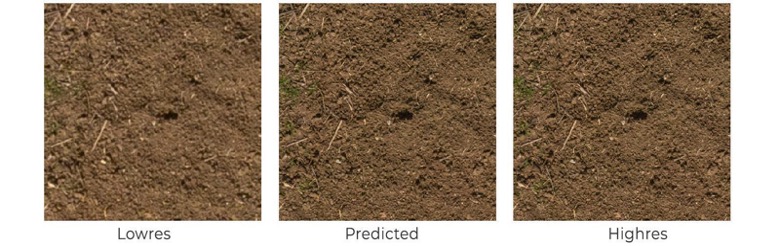
Super-resolution comparison: low-resolution input (left), DCSCN predicted output (centre), ground truth high-resolution reference (right). The predicted output recovers leaf edge detail and texture lost in the low-resolution input, enabling reliable detection on imagery that would otherwise be too coarse.
The model selection process produced an important finding beyond the scores. Two of the six approaches tested scored well on technical measures but failed a visual inspection: both introduced false colours and artificial textures into the upscaled images. For a system that relies on colour and texture to tell weed species apart, an image enhancer that invents visual detail it was not given is worse than useless. DCSCN was selected not only because it scored best, but because it was the only model that consistently produced clean, faithful output across all test images.
The reason DCSCN outperformed the alternatives is that it preserves the original pixel detail from the low-quality input rather than filling in gaps with generated content. This is critical for weed detection: the AI needs to see what is actually in the field, not what a generative model guesses might be there.
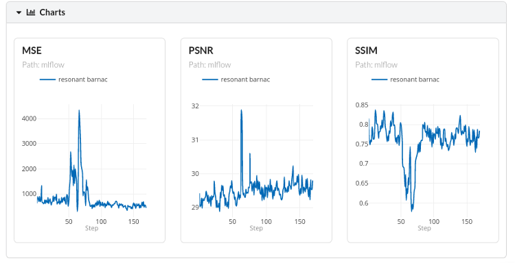
Super-resolution model comparison across six approaches: MSE (lower is better), PSNR, and SSIM (higher is better). DCSCN produces the best combination of all three metrics and, critically, the cleanest visual output. GAN-based models scored well on metrics but introduced colour artifacts that disqualified them from use in a detection pipeline.
The practical implication is a two-stage pipeline for lower-quality imagery: DCSCN first reconstructs the image to a usable resolution, and the detection or segmentation model then runs on the upscaled output. This extends the system’s operational range to higher-altitude survey flights, lower-cost drone platforms, and non-ideal flying conditions, without requiring a second low-altitude pass over the entire field.
Object Detection: Locating and Counting Weeds with YOLOv5
Object detection is the workhorse of weed mapping because it produces the most directly actionable output for precision spraying: a bounding box around each detected plant, labelled with the species and the model’s confidence score. A variable-rate sprayer can be programmed from a map of box centres and class labels in a way that it cannot be programmed from pixel-level class maps alone.
Three AI detection models were tested against the same real drone imagery. Faster RCNN scored 0.643, a strong result that confirmed the task was achievable. YOLOv4 scored 0.579, slightly lower but faster to run. YOLOv5 Large scored 0.661, the best result across all three, and was selected for the final pipeline.
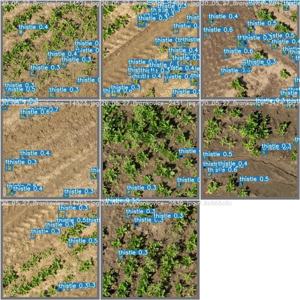
YOLOv5 Large detection output on drone imagery of an arable field. Each bounding box identifies a single plant instance with its class label and confidence score. Thistle weeds (shown in red) are correctly distinguished from the surrounding beetroot crop.
The model was first trained on a large general image library, then specialised on the drone-captured crop and weed images. Techniques including flipping, colour shifting, and image compositing were applied to expand the training set artificially, helping the model generalise to new field conditions. The larger YOLOv5 variant was chosen over smaller versions because distinguishing visually similar species at the leaf level requires greater model capacity.
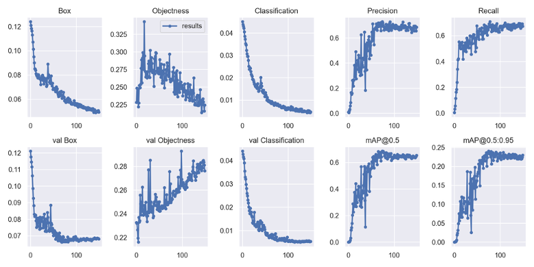
YOLOv5 training curves over 100 epochs. Box loss and classification loss decrease steadily, and [email protected] continues to improve throughout the full training run, indicating that the model has not reached saturation and could benefit from additional annotated examples.
The training graphs show the model improving steadily without signs of overfitting to its training images. Detection accuracy was still rising at the end of training, indicating that more annotated examples, rather than longer training time, is the clearest path to further improvement.
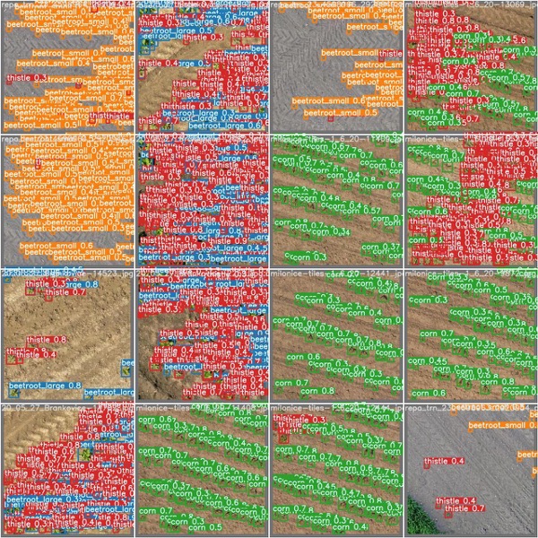
Multi-class detection output showing beetroot (green), maize (blue), and thistle (red) detections in a mixed field tile. The model correctly distinguishes the morphologically similar species across different sizes and densities.
Semantic Segmentation: Mapping Every Field Pixel as Crop or Weed
Where object detection draws a rectangle around each plant, semantic segmentation classifies every individual pixel in the image. The output is a colour-coded mask in which each pixel carries a label: crop, weed, soil, or background. This gives a fundamentally different kind of information, not just the location of weeds but the precise extent and coverage of infestations, which is valuable for calculating infestation density and for identifying contiguous weed patches that cannot be captured adequately by individual bounding boxes.
The semantic segmentation pipeline: image tiles are fed through U-Net EfficientNet for per-pixel classification and Mask R-CNN for instance-level segmentation. Outputs are stitched into field-scale infestation maps.
Three variations of the segmentation model were tested, each using a different underlying feature extractor optimised for speed, boundary precision, or overall accuracy. The EfficientNet version produced the best results and was selected as the primary model. Its design preserves fine spatial detail throughout the network, which is important for accurately tracing the edges of individual plants at the pixel level.
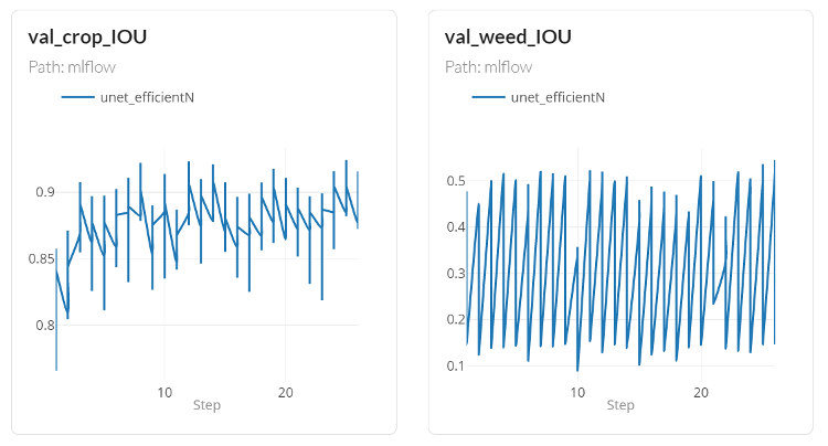
U-Net EfficientNet segmentation results by class. Crop pixels (beetroot, maize) achieve IOU consistently above 0.88, reflecting the relative visual uniformity of cultivated crop rows. Weed pixels achieve an IOU between 0.3 and 0.5, reflecting the greater visual variability and sparse occurrence of thistle in these fields.
The IOU results reveal a meaningful pattern. Crop segmentation is strong: IOU values of 0.88 and above for both beetroot and maize reflect the visual regularity of cultivated plants grown in rows at controlled spacing. Weed segmentation is harder. Thistle in a real arable field appears at variable growth stages, in isolated plants and clusters, partially occluded by crop canopy, and without the spatial regularity that makes crop rows easy to identify from above. IOU between 0.3 and 0.5 for weed pixels is a genuine reflection of that difficulty, not a modelling failure.
Improving weed segmentation IOU is primarily a data problem. A model that has seen more examples of thistle at different growth stages, lighting conditions, and infestation densities will learn a richer visual representation of the class. The active learning pipeline described above is precisely the mechanism for accumulating those examples efficiently as the system is deployed across more fields.
Instance Segmentation: Species-Level Precision with Mask R-CNN
Semantic segmentation assigns each pixel to a class, but cannot distinguish individual plant instances within the same class. A dense weed patch in a semantic segmentation output appears as a single connected region of weed pixels, with no information about how many individual plants it contains. Instance segmentation solves this by simultaneously assigning each pixel to a class and associating it with a specific plant instance. Every thistle in the image is labelled as a distinct object with its own mask.
The model used for this task, Mask R-CNN, goes a step further than standard object detection. Rather than placing a box around each plant, it traces the exact pixel outline of every individual plant. Each weed in the image has its own precise boundary, enabling the counting of individual plants and the measurement of their exact coverage area.
Training this model required more detailed annotation than bounding boxes alone: human annotators drew polygon outlines around each plant, which is significantly more time-consuming per image. This made the prioritisation of active learning especially valuable, ensuring that every annotation hour was spent on the images that would deliver the greatest improvement to the model.
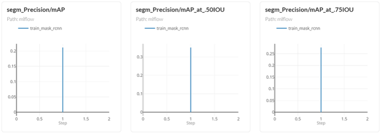
Mask R-CNN instance segmentation metrics at varying IoU thresholds. Performance is strongest at the standard [email protected] threshold, reflecting reliable coarse instance boundaries, with scores falling at stricter thresholds ([email protected]) where tighter pixel-level mask accuracy is required, a known challenge for overlapping vegetation imagery.
The results show that the model reliably identifies the locations of individual plants. Accuracy drops when the scoring standard requires near-perfect pixel outlines, a known challenge when plants overlap or cast shadows on one another. For precision spraying, knowing approximately where each weed is located is what matters; sub-centimetre boundary accuracy is not needed to direct a spray nozzle.
Image segmentation provides what the other two approaches cannot: an individual plant count within each detected zone. Knowing that a field section contains four isolated thistle plants versus forty plants in a dense patch changes the spraying response entirely. Four isolated plants call for targeted spot treatment; forty in a cluster require coverage across the full patch. Together, the three pipelines provide everything needed to design spraying plans matched to what is actually in each field.
Results: Three Pipelines, Three Honest Verdicts
The table below summarises how each model performed. For weed detection, the score reflects the fraction of plants correctly identified. For pixel mapping, the score measures how closely the model’s outlined areas match actual crop and weed coverage. For image enhancement, the scores measure how closely the upscaled output resembles the true high-resolution reference.
| Model | Task | Primary Metric | Score | Notes |
|---|---|---|---|---|
| YOLOv4 | Object Detection | [email protected] | 0.579 | Real data training |
| Faster RCNN | Object Detection | [email protected] | 0.643 | Real data training |
| YOLOv5L ★ | Object Detection | [email protected] | 0.661 | Best detector; real data |
| YOLOv5 (synthetic) | Object Detection | [email protected] | 0.079 | Trained on synthetic only |
| U-Net EfficientNet ★ | Semantic Seg. | IOU (crop) | 0.88+ | Weed IOU 0.3–0.5 |
| Mask R-CNN | Instance Seg. | [email protected] | — | Species-level boxes |
| DCSCN + Skip Conn. ★ | Super-Resolution | PSNR / SSIM | Best | Best metrics; no color artifacts |
The detection results establish two clear findings. First, YOLOv5 Large is the strongest weed detector tested, correctly identifying roughly two-thirds of plants in real drone imagery. Second, the eight-fold gap between real-data and synthetic-data performance confirms that computer-generated training images cannot substitute for real photographs. The visual difference between a synthetic render and an actual drone image is simply too large for a model to bridge on its own.
The pixel-mapping results reflect the true task difficulty. Classifying the main crop area scored above 0.88, a strong result for real agricultural imagery. Weed accuracy scored between 0.3 and 0.5, reflecting how visually variable isolated thistle plants are compared with uniform crop rows. This is not a failure: it is an honest measure of what the current dataset allows. Each additional annotation cycle through the active learning system is expected to improve this figure.
| Results at a Glance |
| YOLOv5 Large: [email protected] = 0.661 · Best object detector · Real drone imagery |
| Synthetic data test: [email protected] = 0.079 · 8.4× gap confirms real annotation is essential |
| U-Net EfficientNet: Crop IOU ≥ 0.88 · Weed IOU 0.3–0.5 · Genuine per-pixel mapping |
| Mask R-CNN: Individual plant instance detection and counting at the species level |
| DCSCN Super-Resolution: Best PSNR and SSIM · Lowest MSE · Enables low-quality imagery processing |
From Model to Field: Herbicide Reduction and the Path to Deployment
Precision spraying reduces chemical use in direct proportion to weed coverage: a field where 10% of the area is infested, in principle, needs only 10% of the herbicide a broadcast programme would apply. The models in this project are not yet at full recall, and turning detection maps into spraying instructions requires compatible application hardware. That said, independent patch-spraying trials in UK and European arable fields consistently report 50-80% reductions in herbicide use with equivalent weed control outcomes.
Reduced herbicide use matters beyond the input bill. UK and EU regulations on pesticide use are tightening, and food processors and retailers increasingly ask suppliers to demonstrate lower chemical use. Weed maps from this pipeline provide a field-by-field record of exactly where chemicals were and were not applied — something a broadcast spray programme cannot produce.
Turning the pipeline into a field product means assembling individual image predictions into complete GPS-aligned field maps and running image enhancement automatically before detection on every incoming flight. The active learning system already in place handles continuous improvement. Each new field deployment adds imagery from new conditions, and the most informative examples are routed back to annotators to retrain the model. A system that improves with every field it visits is fundamentally different from a one-time release.
About the Project
Omdena completed this project, applying computer vision and deep learning to drone imagery of arable fields to detect, classify, and map weed species at the individual plant level. A global team of AI engineers worked across four parallel streams: active learning annotation, object detection, semantic and instance segmentation, and super-resolution image enhancement.
The work delivered three working computer-vision pipelines and an active-learning infrastructure built to improve as the system encounters new fields and conditions continually. Omdena’s collaborative approach brought together computer vision specialists, agricultural experts, and annotation engineers — from data labelling through to a deployable field intelligence system.
If you are building drone-based crop intelligence systems, evaluating computer vision for precision agriculture, or looking to reduce chemical input costs through smarter field mapping, reach out to the Omdena team to discuss how this approach can apply to your context.