Weed and Crop Detection with Semantic vs Instance Segmentation
Learn how semantic and instance segmentation perform in real-world weed and crop detection for smart, data-driven agriculture.

This study compares semantic and instance segmentation approaches for weed and crop detection in real agricultural conditions. The results show that semantic segmentation delivers more reliable performance when data is limited and plant shapes vary widely, enabling more accurate weed mapping and targeted herbicide application. By reducing chemical use, lowering operational effort and improving decision precision, the findings support scalable, data driven and environmentally sustainable farming practices.
Introduction
Precision weed and crop detection is essential for automated weeding and targeted herbicide application in modern agriculture. As farming operations scale, manual identification of weeds becomes increasingly impractical, while blanket herbicide use raises costs and accelerates environmental degradation. Computer vision enables pixel-level analysis of aerial and ground-based imagery, allowing interventions to be applied only where necessary and reducing overall chemical usage.
In this context, Omdena collaborators worked with SkyMaps Agrimatics to explore machine learning and computer vision approaches for weed and crop detection. This article compares semantic segmentation and instance segmentation methods, examining their performance, data requirements and practical trade-offs in real agricultural settings. By analysing how each approach handles field variability, plant morphology and dataset limitations, the study aims to identify which segmentation strategy is better suited to improving efficiency, reducing herbicide use and supporting sustainable, data-driven farming practices.
Challenges of Weed Control
Herbicides are widely used to control invasive weeds. Aggressive species such as Persicaria perfoliata (mile-a-minute weed) can spread rapidly, crowding out native plants and reducing yields. While herbicides support productivity, their overuse contaminates soil and water and poses risks to ecosystems and human health.
To limit chemical use, modern farms are adopting agricultural robotics. Autonomous drones can scan large fields, capture aerial imagery and selectively apply herbicides, but they rely on precise GeoJSON coordinates to guide spraying. In large-scale farms, manually reviewing thousands of orthomosaic image tiles to distinguish weeds from healthy crops is labour-intensive, time-consuming and error-prone.

Orthomosaic image acquired by UAV of sugar cane plantations and its human-generated ground truth. Source
The orthomosaic image above illustrates how human‑generated ground truth masks identify weed and crop regions in sugar cane plantations. These annotated maps serve as the training data for computer vision algorithms.
AI and Computer Vision for Weed Detection
Recent advances in artificial intelligence and agricultural technology, particularly computer vision, allow farmers to automate the process of weed mapping. Machine learning models trained to distinguish crops from weeds can generate precise GeoJSON coordinates far more quickly and consistently than manual methods. Drone-based computer vision pipelines have already demonstrated how high-resolution imagery can be translated into accurate weed maps, enabling selective spraying and large-scale automation in real farm environments. These outputs can be evaluated and refined to ensure herbicide application is highly targeted, reducing the overall use of toxic chemicals.
By minimising unnecessary spraying, such systems lower operational costs and support sustainable farming practices by protecting soil health and biodiversity. This shift toward targeted, data-driven weed control aligns with broader developments in AI-driven agriculture, where machine learning supports precision input application, crop monitoring, and sustainable farm management.When combined with other predictive tools, AI-based weed detection also enables more informed decisions around planting schedules, irrigation planning and crop protection strategies.
Segmentation Models
1. History – Pre Neural Networks
Before the advent of deep learning models, scientists used approaches like the Semantic Texton Forest and Random Forest‑based classifiers for object class segmentation. Later, as the use of Deep Neural Networks (DNN) advanced for image recognition, Convolutional Neural Networks (CNN) achieved enormous success in segmentation problems.

Early attempts at Semantic Segmentation – Source: Shotton et. al circa 2008
The figure above illustrates early attempts at semantic segmentation from Shotton et al. circa 2008, serving as a historical baseline for the evolution of more sophisticated methods.
One popular deep learning approach was patch classification, where each pixel was separately classified into classes using a patch of images around it. The main motivation for using patches was that classification networks typically have fully connected layers and therefore require fixed‑size images. Semantic segmentation refers to the process of linking each pixel in an image to a class label. For example, in the image below, each red pixel is associated with the “weed” class and each green pixel with the “crop” class.

Source: Sugar Beets dataset
This example from the Sugar Beets dataset shows how semantic segmentation assigns red pixels to weeds and green pixels to crops, illustrating the goal of pixel‑wise classification.
In 2014 Long et al. popularised the use of segmentation without any fully connected layers in their academic paper Fully Convolutional Networks for Semantic Segmentation. This improved the segmentation maps generated for images of any size, and the model performed faster compared to the patch classification approach. Almost all the subsequent state‑of‑the‑art approaches to semantic segmentation adopted this paradigm.

convolutional networks Source
Later, different variations of the segmentation model architecture proposed by scientists evolved to tackle the segmentation problem. The following is an overview of some of these models
This figure illustrates how fully convolutional networks perform segmentation by highlighting different regions within an image. It underscores the transition from patch‑based classification to end‑to‑end dense prediction.
2. U‑Net
U‑Net was originally developed by Ronneberger et al. for Biomedical Image Segmentation. The U‑Net architecture consists of two main parts or paths: the encoder and the decoder. The first path is known as the contraction path, which is used to obtain the context of the image. The encoder consists of a stack of convolutional layers along with max‑pooling layers. The decoder of the second path is also known as the symmetric expanding path, which is used for transposed convolutions and precise localisation. U‑Net is thus a fully connected convolutional layer as it does not contain any dense layer and has only convolutional layers. The ability of U‑Net to precisely localise the borders present in the image is because it performs classification on every pixel: the input and the output have the same size.

U‑Net architecture Source
The illustration above outlines the U‑Net architecture: its contracting path captures context while the symmetric expanding path enables precise localisation, culminating in pixel‑wise segmentation.
3. MobileNet
MobileNet is a variation of U‑Net with a streamlined architecture. It significantly reduces the number of parameters when compared to a network with regular convolutions of the same depth. This results in lightweight deep neural networks that are ideal for mobile and embedded vision applications that operate “on the edge” and may have limited processing power.
4. EfficientNet
EfficientNet is a convolutional neural network architecture and scaling method that uniformly scales all dimensions of depth, width and resolution using a compound coefficient. Unlike other conventions that arbitrarily scale these factors, the EfficientNet scaling method uniformly scales the dimensions using a set of fixed scaling coefficients. The compound scaling method is justified by the intuition that if the input image is bigger, then the network needs more layers to increase the receptive field, and more channels to capture more fine‑grained patterns on the bigger image.
5. SegNet
SegNet: A Deep Convolutional Encoder‑Decoder Architecture for Image Segmentation (Badrinarayanan et al.) is another iteration of semantic segmentation motivated by reducing training time through memory optimisation. Architectures that store the entire encoder network feature maps perform best but consume more memory during inference time. SegNet, on the other hand, is more efficient since it only stores the max‑pooling indices of the feature maps and uses them in its decoder network to achieve good performance. On large and well‑known datasets SegNet performs competitively, achieving high scores without memory versus accuracy trade‑offs associated with achieving good segmentation performance.
6. Mask R‑CNN
In 2017 He et al. introduced a new type of segmentation, instance segmentation, with the publication of Mask R‑CNN. Mask R‑CNN is an extension of the Object Detection algorithm Faster R‑CNN with an extra mask head. The extra mask head allows pixel‑wise segmentation of each object and extraction of each object separately without any background (which is not possible by semantic segmentation). Mask R‑CNN can separate different objects within images or a video. It identifies the object bounding boxes, classes and masks within an image.

architecture of Mask R‑CN Source
The diagram illustrates the overall architecture of Mask R‑CNN, showing how region proposal networks, classification heads and the mask head work together to identify each object and extract its mask.
Evaluation of Semantic Segmentation Models
Recall that the task of semantic segmentation is simply to predict the class of each pixel in an image.

The above image provides an example output from a semantic segmentation model, where each pixel is assigned a class label.
Common ways to evaluate semantic segmentation model performance include:
Intersection Over Union (IoU)

IoU evaluation figure
IoU is the area of overlap between the predicted segmentation and the ground truth divided by the area of union between the predicted segmentation and the ground truth. This metric ranges from 0 to 1 with 0 signifying no overlap and 1 signifying perfectly overlapping segmentation. For binary (two classes) or multi‑class segmentation, the mean IoU of the image is calculated by taking the IoU of each class and averaging them. IoU is generally considered the leading indicator for a semantic segmentation model’s performance.
This graphic depicts the IoU calculation by showing the overlapping area and total union area between predicted and ground‑truth masks.
Dice‑Coefficient
Dice coefficient is a spatial overlap index and a reproducibility validation metric. It has scores ranging from 0 (which indicates no spatial overlap between two sets of binary segmentation results) to 1 (which indicates complete overlap). It is used to measure the similarity of two samples. It is calculated as 2 × the Area of Overlap divided by the total number of pixels in both images.
Pixel Accuracy
Pixel accuracy is the most basic metric which can be used to validate segmentation results. Accuracy is obtained by taking the ratio of correctly classified pixels with regard to the total pixels:
Pixel Accuracy = (TP + TN) / (TP + TN + FP + FN)
A disadvantage of using pixel accuracy alone is that the result might look good if one class overpowers the other. For example, if the background class covers 90 % of the input image, we can get an accuracy of 90 % by just classifying every pixel as background.

Pixel Accuracy formula figure
The formula above demonstrates how pixel accuracy is computed from counts of true positives (TP), true negatives (TN), false positives (FP) and false negatives (FN).
Frequency Weighted IoU
This is an extension over the mean IoU which we discussed and is used to combat class imbalance. If one class dominates most parts of the images in a data set (for example background), it needs to be weighed down compared to other classes. Thus, instead of taking the mean of all the class results, a weighted mean is taken based on the frequency of the class region in the data set.
F1 Score

F1 Score figure
F1 score is a metric popularly used in classification; it can also be used for segmentation tasks to deal with class imbalance.

Explanation of How F1 Score is Derived
These diagrams explain how the F1 score is derived from precision and recall, illustrating its usefulness for handling class imbalance.
Evaluation of Instance Segmentation Models
Instance segmentation models are more complicated to evaluate. Semantic segmentation models output a single segmentation mask, whereas instance segmentation models produce a collection of local segmentation masks describing each object detected in the image. For that reason, evaluation methods for instance segmentation are similar to those of object detection, except that we calculate IoU of masks instead of bounding boxes.

Visual Comparison of Semantic Segmentation vs Instance Segmentation. – Source: Jeremy Jordan
The comparison above contrasts semantic segmentation, which assigns every pixel to a class, with instance segmentation, which differentiates individual objects even within the same class.
Average Precision
Average precision computes the average precision value for recall values over 0 to 1.
Mean Average Precision (mAP)
The mAP is the mean of the average precision scores and is used as a metric for instance segmentation to measure how accurate the predictions are at the pixel level. Values for mAP evaluation lie between 0 and 1.

The area under this Precision-Recall curve gives you the “Average Precision”. Source
In this figure the area under the precision–recall curve corresponds to the average precision, which is averaged across recall levels to compute mean average precision (mAP).
Data Set Requirements
1. Semantic Segmentation
a) Masks and Image Dimensions
Semantic segmentation requires an associated PNG file with a mask for each image. The mask assigns each pixel to its class using a specific RGB colour. This pairing ensures that the model learns from both the image and the corresponding labelled mask.

Masks and Image Dimensions
Input images must be of identical height and width. The minimum effective dimensions for training are 512×512 pixels. Larger datasets with many files may cause memory issues on GPUs, so our engineers experimented with smaller images (256×256 pixels). We observed that input size significantly influences key performance metrics, notably Intersection over Union (IoU).

Dimentions Mesurments
b) Directory Structure
Your dataset directory structure should be organised consistently so that each image file has an identically named mask placed in the corresponding train/test/validation masks directory. This prevents filename conflicts and ensures the data loader can correctly pair images and masks.

Directory Structure
We obtained high‑quality weed/crop semantic segmentation maps using a subset of the publicly available Sugar Beets data set produced by the University of Bonn.
2. Instance Segmentation
a) COCO Annotations and Image Dimensions
Mask R‑CNN requires training data to be annotated in the COCO format. This annotation style traces the outline of each object instance using a series of (x, y) coordinates, providing pixel‑specific locations for each instance. Each instance is assigned its own colour in the translucent mask.

COCO Annotations and Image Dimensions
Input images can have varying dimensions such as 1024 × 768 pixels. COCO‑annotated images produce a single JSON file irrespective of the number of images annotated.
Example COCO annotation file below:

COCO annotation file
b) Directory Structure and Synthetic Data
The instance segmentation dataset should be structured so that images and their COCO annotations reside in an organised directory. A clear directory layout assists in loading the data correctly.

Directory Structure
Because large, publicly available COCO datasets of weed vs crop were not available, we constructed our own using synthetic data generation. This process involved hand‑labelling samples with pixel‑wise COCO coordinates for weeds and crops, extracting the foreground objects, and programmatically pasting them onto randomly selected soil backgrounds. Various augmentations (rotation, scaling, etc.) expanded our sparse baseline dataset.

Omdena’s project pipeline for Synthetic Dataset Generation
Model Research Overview
1. Semantic Segmentation Models
In our research we explored several semantic segmentation architectures: a baseline U‑Net, U‑Net variants with EfficientNet backbones and MobileNet backbones. EfficientNet uses compound scaling—that is, it scales depth, width and resolution together to achieve a balanced architecture. This design delivers performance improvements compared to other convolutional networks. MobileNet employs depth‑wise separable convolutions, dramatically reducing complexity, cost and model size. Lighter models are attractive for real‑time and embedded applications, although our MobileNet variant exhibited lower performance than the EfficientNet U‑Net and the baseline U‑Net due to its reduced capacity.
2. Instance Segmentation Models
We also trained and evaluated instance segmentation networks using Mask R‑CNN. Unlike semantic segmentation, Mask R‑CNN outputs individual masks for each detected object. Our experiments used ResNet‑50 and ResNet‑101 as backbone CNNs together with Feature Pyramid Networks. The model employs selective search to generate region proposals, and we applied batch normalisation to mitigate over‑fitting and under‑fitting. Between the two backbones, Mask R‑CNN with ResNet‑101 performed better than the ResNet‑50 variant: the smaller model yielded higher loss and lower mean average precision (mAP). Instance segmentation results were also more variable across categories. Small plants were particularly challenging, and mis‑detections often stemmed from bias rather than resolution limitations.
3. Model Performance
The Dice Coefficient shows the superior ability of U‑Net‑EfficientNet in segmenting crops/weeds compared to the other methods. Baseline U‑Net shows better results as a multi‑class segmenter (with 0.9367 IoU).
Overview of Model Performance Metrics Across All Segmentation Tasks
1. Semantic Segmentation Performance
| Model Name | Dimensions | IOU (Crop / Weed) | Dice Coefficient (Crop / Weed) |
|---|---|---|---|
| U‑Net | 896×896 | 0.9367 / 0.8079 | 0.8934 / 0.8934 |
| U‑Net (EfficientNet‑B0) | 768×768 | 0.8574 / 0.4580 | 0.9216 / 0.6198 |
| U‑Net | 512×512 | 0.85 / 0.25 | 0.92 / 0.40 |
| U‑Net (MobileNet) | 256×256 | 0.5630 / 0.0545 | 0.4856 / 0.0427 |
2. Instance Segmentation Performance
| Model Name | Dimensions | mAP |
|---|---|---|
| Mask R‑CNN (ResNet‑101) | 512×512 | 0.590 |
| Mask R‑CNN (ResNet‑50 + FPN) | 1024×768 | 0.396 |
Analysis of Results
1. Comparing Performance
Across our experiments, semantic segmentation models consistently outperformed instance segmentation for distinguishing crops from weeds. Two factors drove this result: first, the semantic segmentation dataset was considerably larger than the instance segmentation dataset; second, weed and plant sizes vary greatly, which complicates instance segmentation. Because the COCO dataset available for weeds and crops was much smaller than our baseline segmentation dataset, Mask R‑CNN models suffered from limited training samples.
2. Data Limitations
A key obstacle to improving Mask R‑CNN performance was the scarcity of high‑quality COCO data. While a robust, balanced semantic segmentation dataset existed (such as the Sugar Beets set), comparable COCO datasets for crops and weeds were not readily available. Building a custom COCO dataset required painstaking pixel‑by‑pixel labelling, a labour‑intensive task that was impractical within our project’s timeline.
3. Difficulty of Weed Contours
Even with synthetic data generation techniques, the COCO annotation style proved poorly suited to weeds. Weeds often have wispy, irregular contours, making it difficult to draw precise polygonal annotations around each plant. This complexity undermines both natural and synthetic COCO generation, limiting the utility of instance segmentation for these species.

The weed input image and corresponding mask. Source: Sugar Beets dataset
The pair above shows the original weed image alongside its corresponding mask from the Sugar Beets dataset, illustrating how ground truth labels delineate weed regions.
Conclusion
In this project, we evaluated multiple segmentation techniques and dataset requirements for detecting crops and weeds from drone imagery. The results show that semantic segmentation consistently outperformed instance segmentation, largely due to a larger and more balanced training dataset and the high variability in plant sizes and shapes that limited Mask R-CNN performance. Irregular weed morphology further reduced the effectiveness of instance segmentation models.
Overall, the findings emphasise the importance of data quality and choosing the right model for reliable weed detection. Accurate crop and weed segmentation not only enables targeted herbicide application but also supports sustainable farming by optimising resource use, When combined with multispectral plant-health analysis, segmentation outputs can further guide irrigation, nutrient management, and early stress detection at field scale. reducing chemical dependency and lowering environmental impact as data-driven agriculture becomes more widely adopted.
If you want to apply drone imagery and computer vision to precision weed management and cut chemical use, Omdena helps translate AI research into practical, field-ready farming solutions. Explore how this approach can scale across real agricultural landscapes.