
AI Solar Energy Yield Forecasting: How Operators Predict and Protect Generation Revenue
Discover how AI solar yield forecasting improves forecast accuracy, reduces revenue loss, and helps operators optimize solar generation.
June 9, 2026
10 minutes read
A 50 MW plant operator reviews Q3 results: no faults, no incidents, availability above 98 percent for the quarter. Revenue still came in 9 percent below projection. The shortfall traced not to hardware failure but to forecast error: maintenance had fallen outside peak generation windows, and trading positions had been sized against generation that never arrived.
Most operating solar plants still use Numerical Weather Prediction (NWP)-based forecasting built for grid balancing rather than revenue maximisation. These tools produce directional accuracy at day-ahead resolution, which is sufficient to keep the grid stable but insufficient for dispatch timing, curtailment execution, or maintenance scheduling. The gap between what the forecast said and what the plant produced is where revenue leaks, and it is rarely attributed to the forecast itself.
This article covers how AI-based yield forecasting closes that gap, what improved forecast accuracy looks like in operational terms, and how to evaluate whether the revenue protection case applies to your portfolio.
How AI Yield Forecasting Works: From Regional Weather to Site-Level Learning
NWP models ingest atmospheric data from weather stations and satellites to produce regional forecasts at 6-hour to day-ahead intervals. For solar generation, this tells an operator whether the day will be sunny or overcast. It does not resolve what happens between 11:00 and 11:15 when a cloud bank arrives, or how a localised weather pattern affecting only their site will alter output across the next trading period.
AI yield forecasting trains on the specific site’s historical generation data, cross-referenced with local irradiance, temperature, humidity, and satellite imagery at short intervals. The model learns how site-specific microclimate patterns repeat, how the plant responds to partial shading and wind-driven cooling, and how soiling affects output through the year. The result is a probabilistic forecast at 15-minute intervals, expressed with confidence bounds that the operator can act on.
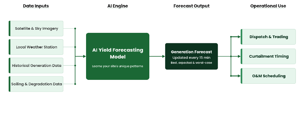
Figure 1: AI yield forecasting process — from data inputs to operational decisions
The operational difference is concrete. A 6-hour NWP forecast provides a directional view: plan maintenance for a low-sun day and rough-size the dispatch position. A 15-minute AI forecast tells an operator that output will drop 18 percent between 13:20 and 14:10, that Wednesday’s cleaning crew costs less lost generation than Thursday’s, and that tomorrow afternoon’s trading position should be reduced. Decisions once made on instinct are now made on data.
That is what makes yield forecasting different from performance monitoring. Performance monitoring identifies the generated output that was lost due to equipment failure. Yield forecasting captures generation that was never planned for because the model indicated it would not come.
What Standard Solar Forecasting Misses and How AI Catches It
NWP models perform reliably at the regional scale and over long time horizons. Their limitations lie in resolution and site specificity, and those limitations fall exactly where solar revenue decisions are made. Below is what standard forecasting consistently misses and what AI-based forecasting detects instead.
Cloud Ramp Events: The 30-Minute Blind Spot
Up to 35 percent of forecast error at high-variability sites is due to cloud ramp events lasting under 30 minutes. On a coastal site, a ramp arriving at 14:00 can drop output from 85 percent to 40 percent of rated capacity within 20 minutes, with no warning in the NWP day-ahead forecast. AI forecasting, trained on local satellite imagery at 5-minute resolution, detects these events early enough to adjust dispatch and curtailment decisions before the ramp arrives.
Soiling and Degradation: Forecasting a Plant That No Longer Exists
5 to 12 percent of forecast underperformance is attributable to soiling and degradation losses that standard models treat as nameplate capacity. AI forecasting incorporates historical soiling curves and real performance data, so the forecast already reflects what the plant is actually capable of producing on a given day, not what it was rated to produce when it was new.
Wind-Cooling Effects: The Uplift NWP Leaves on the Table
A 10 to 20 percent improvement in short-horizon accuracy comes from modelling wind-cooling effects. Inverter and module efficiency improve with lower ambient temperature. AI forecasting captures the output uplift that follows wind events and cold mornings, adding generation to the forecast that standard models miss and that operators currently leave unscheduled.
Seasonal Microclimate Patterns: What Regional Models Cannot See
2 to 4 percent of annual generation is affected by seasonal microclimate patterns that standard forecasts do not model at the site level. Valley shading, coastal fog, terrain-driven cloud, and localised humidity cycles are invisible to regional NWP models but consistently predictable from multi-year site history. AI forecasting learns these patterns and prices them into day-ahead and week-ahead projections.
Post-Maintenance Recalibration: The 30 to 60 Day Revenue Gap
A 30- to 60-day recalibration lag follows major maintenance events under standard forecasting. After a large cleaning cycle or component replacement, the plant is producing at a different level than the model was trained on. AI forecasting continuously recalibrates using live performance data, so the forecast reflects post-maintenance output almost immediately, and operators stop losing revenue during the recalibration window.
Each of these gaps compounds. An operator who loses forecast accuracy across cloud ramps, degradation drift, and seasonal microclimate effects simultaneously is not making small errors in individual decisions. They are making compounding errors across every operational window that forecast data informs.
Real-World Results: AI Forecasting Accuracy at Operational Scale
The gaps described above are not theoretical. Published research across two deployment contexts demonstrates what accuracy improvement looks like when AI replaces NWP-only forecasting at an operational scale.
Utility-scale sites across variable irradiance zones. Industry research comparing AI-based sky-camera forecasting against NWP and simple benchmark methods across utility-scale test sites found a 20 to 30 percent reduction in MAPE for 30-minute ahead forecasts. The accuracy improvement was largest in the 10- to 30-minute forecast window, where cloud ramp events drive curtailment and dispatch decisions, making it the highest-value and most underserved forecast horizon for solar operators managing short-term positions.
A high solar-penetration electricity market. In one of the world’s most solar-penetrated electricity grids, ML-based forecasting was deployed across a portfolio of large solar farms, with outcomes documented in the grid operator’s data. Accuracy improvements were largest for high-variability sites. Improved short-horizon forecasting reduced the balancing reserve costs operators had previously carried to compensate for standard forecast error, translating directly into operational cost reductions across the portfolio.
Across both cases, the improvement was most visible in the same operational windows: short-horizon dispatch decisions, curtailment timing, and scheduling made 24 to 48 hours ahead. These are the windows that standard NWP cannot resolve at the site level and where revenue is determined.
The Revenue Protection ROI
Forecast error converts to revenue loss in three places simultaneously. In energy trading and dispatch, inaccurate forecasts produce mis-sized positions. In PPA and offtake compliance, shortfalls trigger financial penalties. In Operations and Maintenance (O&M) scheduling, maintenance planned against an inaccurate forecast conflicts with peak generation windows, incurring both direct cost and production loss. Addressing all three requires a forecast accurate enough to drive decisions in each window.
| Portfolio Size | Estimated Annual Revenue Protected by AI | Typical Payback Period of an AI System |
|---|---|---|
| 10 MW | $40K–$90K | 1–3 months |
| 50 MW | $200K–$450K | Under 1 month |
| 100 MW | $400K–$900K | Under 1 month |
Payback period based on industry-typical platform costs for each portfolio size. Estimates apply to merchant or partially merchant portfolios at an average of $60 per MWh. Fixed PPA portfolios without performance-penalty clauses will see a lower direct revenue impact, though improved forecast accuracy still reduces O&M scheduling conflicts and improves long-term asset reporting accuracy.
The ROI case compounds beyond the first year. AI forecasting models improve with each operating cycle as site-specific seasonal patterns become more established and variability profiles are captured in greater detail. Accuracy gains in year two are typically 10 to 20 percent better than year one on the same sites, with no additional deployment cost.
Which Portfolios Have the Most Revenue at Risk
Not all portfolios carry equal exposure to forecast error. The signals below identify where yield forecasting has the strongest ROI case. Operators with three or more of these conditions should treat AI forecasting as an immediate operational priority.
Merchant or partially merchant revenue exposure. No guaranteed offtake floor means inaccurate forecasts translate directly to energy trading losses. The revenue consequence of each forecast error is immediate and quantifiable, with no PPA buffer to absorb the shortfall.
PPA contracts with availability or curtailment penalty clauses. Each penalty event that could have been avoided with a more accurate forecast is a direct, quantifiable cost reduction. Portfolios with tight compliance windows gain the most from improved short-horizon accuracy.
Sites in high-variability irradiance zones. Coastal, mountainous, or tropical climates with frequent cloud ramp events produce the largest forecast errors and the largest gains in accuracy for AI models trained on local data. These sites also carry the widest gap between NWP resolution and the operational decisions operators need to make.
Plants over 5 years old with degradation not reflected in the forecast model. Standard forecasts that assume nameplate capacity systematically overestimate output for older assets. AI forecasting incorporates real degradation curves and recalibrates as performance changes, so the forecast reflects what the plant can actually produce.
Portfolios where O&M scheduling depends on generation forecasts. Every panel inspection or maintenance window that conflicts with an unexpected high-generation period incurs both direct labour costs and generation opportunity costs. Accurate short-horizon forecasting eliminates conflicts before they arise, improving both asset availability and O&M efficiency.
Portfolios with fully fixed offtake, low irradiance variability, and no performance-based PPA clauses have the weakest immediate ROI case. AI yield forecasting still improves asset reporting and long-term performance planning for these sites. Still, the revenue protection case builds over a longer horizon than for merchant or high-variability portfolios.
How to Deploy AI Yield Forecasting
AI yield forecasting connects to existing data infrastructure rather than replacing it. Most platforms integrate with existing monitoring and telemetry systems via API, pulling historical generation and real-time inverter data without requiring hardware changes. The deployment process is incremental, and accuracy improvement begins within weeks of the first live forecast cycle.
- Baseline your current forecast error. Pull 12 months of actual versus forecast data and calculate MAPE by site and season to identify where forecast error is costing the most.
- Audit your data availability. Confirm you have at least 12 months of generation history, a sub-hourly weather feed, and inverter-level telemetry before starting vendor evaluation.
- Run a parallel pilot on your highest-variability site. A 60- to 90-day parallel run against your existing forecasting method provides a clean comparison of accuracy before committing to a full rollout.
- Integrate with operational scheduling. A forecast that does not feed actual dispatch, maintenance, and trading decisions does not protect revenue. Confirm integration pathways with your operations team before sign-off.
Operators who run a structured pilot before full deployment typically report faster adoption within operations teams and a cleaner ROI case to present to asset owners.
Conclusion: Where Solar Revenue Is Won or Lost
Yield forecasting is the part of solar operations where revenue is lost without any fault-firing or alert triggering. The equipment performs well, availability is high, and the monitoring dashboard shows nothing wrong. The loss accumulates from dispatch windows missed due to an inaccurate forecast, maintenance that conflicts with peak generation periods, and trading positions sized against generation that never arrives.
As energy markets tighten and PPA structures add more performance and availability clauses, forecast accuracy moves from an operational preference to a commercial requirement. The operators who build that accuracy into their portfolios now will carry a measurable revenue advantage into the next generation of solar asset management.
Omdena deploys AI yield forecasting for solar operators and asset managers across portfolios of all sizes, delivering site-specific generation forecasts and revenue-ranked dispatch recommendations at a fraction of typical development costs. If you are ready to find out how much forecast error is costing your portfolio, get in touch with the Omdena team.