
AI and Satellite Imagery for Crop Health Monitoring at Scale — Omdena Case Study
Discover how AI and satellite imagery help monitor crop health, map fields, and classify crops at scale using Sentinel-2 data.
May 8, 2026
11 minutes read
Executive Summary
Monitoring crop health across thousands of fragmented smallholder fields demands more than field visits. This project built an end-to-end satellite intelligence system capable of detecting individual field boundaries and classifying crop types at the district scale, using only freely available Sentinel-2 imagery and open-source tools. It was validated across Guntur district in Andhra Pradesh and Bellary district in Karnataka, two of India’s primary chilli-growing regions.
The system runs two parallel pipelines. The first uses deep semantic segmentation to delineate field boundaries and compares two architectures: ResUNet-a and FracTAL ResUNet. The second derives crop classification from time-series vegetation index signatures using unsupervised K-means clustering on Google Earth Engine. Together, they produce georeferenced boundary and crop maps without requiring costly on-the-ground sensors.
The Problem with Monitoring Crops at Scale
Governments and agribusinesses need reliable district-level data on which crops are growing, how healthy they are, and how far fields extend. Traditional approaches rely on self-reported surveys, seasonal inspections, or sample-based estimates, all of which are slow, expensive, and difficult to verify across millions of fragmented smallholder plots.
Satellite imagery provides continuous, area-wide coverage, but raw spectral data cannot directly answer agronomic questions. It takes an entire pipeline: acquiring cloud-free images at the right season, computing the right spectral indices, training models that understand field boundaries rather than just land cover, and linking outputs to real-world crop records. Each step introduces failure modes that compound downstream.
The FarmHand project addressed this gap in the context of chilli cultivation in southern India, where fields are small, irregular, and tightly interspersed with other crops. The technical challenge was not classification accuracy alone but building a system robust enough to generalise across diverse field sizes, soil backgrounds, and monsoon-affected observation windows.
Sentinel-2 and Why a Single Snapshot Is Never Enough
The project used Sentinel-2 Level 2A imagery acquired through Google Earth Engine. Sentinel-2 delivers multispectral data at 10-metre resolution with a 5-day revisit cycle, making it the highest-resolution freely available satellite source for field-scale agricultural monitoring. A strict cloud cover threshold of 10 percent was applied during filtering, leaving 15 usable images spanning the November 2019 to March 2020 growing season.
Rather than treating each image independently, the pipeline stacked bands across timestamps to create multi-temporal feature tensors. This temporal depth is what separates crop monitoring from simple land classification. Chilli, mint, and other broadleaf crops have distinct phenological signatures, meaning their spectral response changes in characteristic patterns as they emerge, grow, and senesce. A single snapshot cannot capture this; at times, a series can.
Google Earth Engine handled all cloud masking, atmospheric correction, and index computation at the planetary scale, removing the infrastructure burden from the modelling team. The combined use of GEE for acquisition and Sentinel-2 for sensing made the pipeline replicable across any district in India without additional satellite subscriptions or processing infrastructure.
Ground Truth Quality and the Label Alignment Challenge
Ground truth for this project came from three independent sources, contributing a combined 2,884 chilli records and 1,722 mint records. Across all sources, 14.1 percent of labelled points fell in overlapping zones, introducing spatial ambiguity that had to be resolved before training. This level of inter-source disagreement is typical in agricultural labelling efforts and is rarely discussed in published benchmarks.
Label quality directly constrains what a model can learn. Where sources disagree, the model receives conflicting supervision. The team addressed this by computing agreement statistics across sources and treating high-disagreement zones with reduced confidence during training. This kind of principled handling of label noise is more consequential to downstream accuracy than most architectural choices.
The spatial distribution of ground-truth records also shaped the training design. Labels were geographically concentrated in two districts, limiting the model’s direct exposure to field types in other regions. Generalisability beyond Guntur and Bellary would require additional labelling campaigns, a constraint the team acknowledged and documented explicitly.
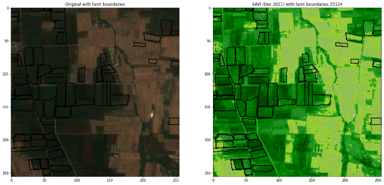
Figure 1: Satellite imagery with ground-truth field boundary overlays across two study districts. Field size variation and irregular plot shapes were core challenges in training the segmentation model.
Benchmarking Two Architectures for Field Boundary Detection
The boundary detection pipeline was evaluated across two deep learning architectures, each building on the same UNet encoder-decoder backbone but differing in how they handle multi-scale context and sparse label supervision.
ResUNet-a: The Baseline Model
Architecture. ResUNet-a uses modified residual blocks, atrous convolutions at multiple dilation rates, and Pyramid Scene Parsing pooling in the bottleneck. It was trained with a multi-task objective producing three simultaneous outputs: an extent mask identifying field interiors, a boundary mask highlighting plot edges, and a distance transform encoding each pixel’s distance to the nearest boundary.
Results and what they reveal. ResUNet-a achieved an F1 of 0.85, which looks strong in isolation. However, its MCC was 0.36, a substantial gap that signals a model biased toward the majority class. MCC accounts for all four confusion matrix cells and penalises the class imbalance inherent in field boundary datasets, where non-boundary pixels vastly outnumber boundary pixels. The F1-MCC discrepancy here is diagnostic: high recall on the dominant class masking poor boundary-pixel sensitivity.
FracTAL ResUNet: Transfer Learning and Attention
Architecture. FracTAL ResUNet replaced the atrous convolution blocks with FracTAL ResNet blocks and added a Tanimoto Attention Layer that re-weights features based on similarity, improving sensitivity to fine-grained boundary signals. The architecture was first pre-trained on densely labelled Netherlands field data, then fine-tuned on the Indian partial labels using a masked loss function that computed gradients only at labelled pixels. Unlabelled regions contributed nothing to parameter updates.
Results and what improved. MCC rose from 0.36 to 0.54 while accuracy held at 0.77, and F1 fell slightly to 0.81. The MCC gain is the meaningful result: the model became substantially better at correctly identifying boundary pixels, which is the operationally critical outcome for downstream field delineation. The small F1 drop reflects higher precision at the cost of slightly lower recall, a trade-off that produces cleaner, less fragmented boundary predictions in practice.
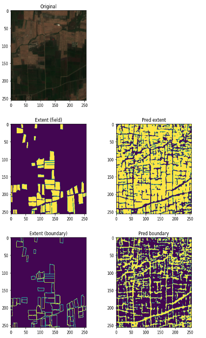
Figure 2: Five-panel comparison showing original imagery, ground-truth extent mask, ground-truth boundary mask, predicted extent, and predicted boundary. The FracTAL model produces boundary predictions closely aligned with the ground-truth overlays.
Model performance summary
| Model | MCC | Accuracy | F1 Score |
|---|---|---|---|
| ResUNet-a | 0.36 | 0.77 | 0.85 |
| FracTAL ResUNet | 0.54 | 0.77 | 0.81 |
From Semantic Masks to Field Instances
Semantic segmentation produces pixel-wise predictions: this pixel is a boundary, that pixel is field interior. Field delineation requires instance segmentation: this contiguous region is one specific field. Converting from semantic to instance is a non-trivial post-processing step that the project handled using the Higra library’s watershed segmentation algorithm.
Watershed segmentation treats the predicted boundary confidence map as a topographic surface, then floods it from seed points to identify catchment basins corresponding to individual fields. The quality of instance outputs depends directly on the quality of boundary predictions. Fragmented boundaries produce over-segmentation; thick or blurry boundaries merge adjacent fields into one instance. This is why boundary MCC matters more than F1: poor boundary sensitivity leads to unusable field maps, regardless of how sophisticated the instance segmentation step is.
The resulting field-instance maps assign each delineated plot a unique identifier and explicit geometric boundaries. Each delineated plot becomes an addressable spatial unit: it can be linked to farmer records, incorporated into district-level acreage estimation workflows, or used as the spatial foundation for any downstream system that needs to reason about individual fields. Field delineation is the enabling layer; everything built on top of it inherits its precision.
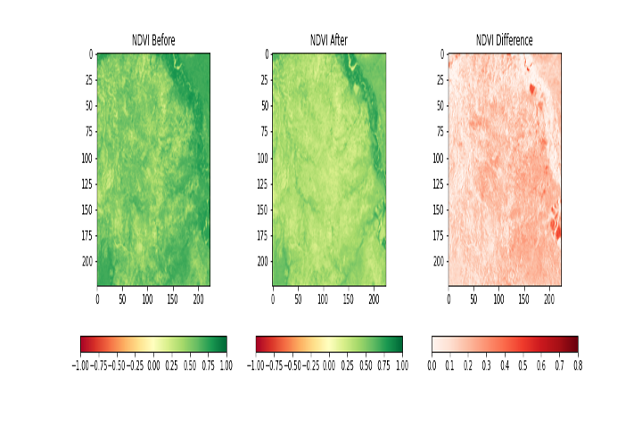
Figure 3: NDVI before, after, and difference panels across the growing season. Temporal changes in vegetation index values are the primary signal used for crop classification and health monitoring.
Identifying Crop Types Without Labelled Training Data
That enabling layer tells you where every field is. It does not tell you what is growing in it. A second pipeline, running on the same Sentinel-2 time-series, answers that question using a different signal representation and an entirely unsupervised approach. While the boundary detection model requires labelled training data and transfer learning, the crop classification pipeline requires neither, making it immediately replicable in any region with satellite coverage.
Index computation and feature engineering
Feature vectors. For each pixel, the system computed four indices at each timestamp: NDVI, EVI, SAVI, and NDWI. Stacked across 15 available dates, this produced a 60-dimensional feature vector per pixel capturing the full spectral-temporal signature of whatever was growing there. This temporal depth is the critical ingredient: a single date cannot reliably distinguish chilli from other broadleaf crops, but a phenological time series encoding how reflectance evolves through the growing season can.
Why these indices? NDVI captures general vegetation density. EVI reduces atmospheric noise and soil background effects at high canopy density. SAVI further corrects for soil reflectance in areas with sparse cover. NDWI is sensitive to canopy water content, adding a dimension that pure greenness indices miss. Together, they provide complementary spectral perspectives on crop condition at every timestamp.
Unsupervised clustering on GEE
K-means with k=3. The feature vectors were clustered on Google Earth Engine using three clusters, reflecting the primary land cover categories in the study area: chilli, other crops, and non-agricultural land. Cluster centroids were then matched to crop types using available ground truth records, so the unsupervised output gains a human-interpretable label without additional annotation effort.
Scale advantage. K-means requires no labelled training data, making it immediately replicable to any new district with Sentinel-2 coverage. GEE handled both the index computation and clustering at the planetary scale, enabling the entire classification component to run without any local compute infrastructure. A new district can be processed end-to-end in under a day.
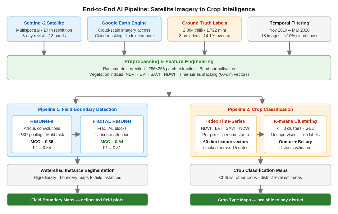
Figure 4: End-to-end system pipeline from Sentinel-2 acquisition through preprocessing, boundary detection, and crop classification to final georeferenced output maps.
Together, the two pipelines produce a single georeferenced inventory: every field in a district is identified by location, extent, and crop type. That complete spatial picture is what makes district-level acreage estimation, targeted advisory services, and crop insurance verification all possible from the same freely available dataset.
Partial Labels, Transfer Learning, and Why Benchmarks Mislead
A consistent theme across this project was the gap between benchmark accuracy and operational usefulness. Standard segmentation benchmarks assume dense, consistent labelling. Indian smallholder field data provides neither. Labels are partial, spatially concentrated, and collected through methods of varying precision. Any model trained naively on such data will produce biased estimates of its own performance.
The project’s use of masked loss functions during fine-tuning is technically straightforward but uncommon in applied agricultural AI. It means gradients propagate only through pixels with confirmed labels, preventing the model from learning false negatives in unlabelled regions to be treated as genuine negatives. Combined with pre-training on European data where dense labels were available, this gave the model a strong prior for what field boundaries look like before it encountered the sparse Indian supervision.
The lesson generalises beyond this project. In any satellite-based agricultural AI system deployed on smallholder land, the bottleneck is almost always label quality, not model capacity. Architectural improvements have diminishing returns when the training signal is noisy. Investment in verified ground truth, even with reduced spatial coverage, yields greater gains than switching between deep architectures.
What This System Makes Possible
India cultivates chilli across roughly 800,000 hectares annually, with Andhra Pradesh alone accounting for nearly a third of national production. The system built here can produce a complete georeferenced crop map for an entire district in under a day of computing time, using no satellite subscriptions, no ground sensors, and no field staff beyond the initial label collection. These are the concrete outcomes it enables.
- State and district agricultural departments can produce verified acreage estimates without relying on farmer self-reporting, using the field boundary maps as the spatial foundation. This replaces slow seasonal surveys with continuous, satellite-derived inventory.
- Agribusinesses and input suppliers can use crop classification maps to target advisory services, seed distribution, and procurement planning to the specific fields growing the crops they serve, reducing outreach waste and improving service uptake.
- The temporal NDVI and EVI signals produced by the pipeline are directly usable for stress monitoring, irrigation advisories, and crop insurance verification. Downstream applications that need to know where fields are and what is growing can be built on top of the outputs without re-running the ML components.
- New districts can be onboarded by collecting a few hundred verified ground truth labels and running the pipeline. Sentinel-2 data is free globally, GEE scales the computation, and the predicted boundary maps can themselves serve as annotation seeds for subsequent labelling campaigns.
- The methodology for partial-label training and cross-domain transfer is replicable beyond Chilli. Any crop grown in fragmented, smallholder plots with available Sentinel-2 coverage can be addressed using the same pipeline architecture and engineering choices.
About the Project
This project was completed by Omdena in collaboration with FarmHand, focusing on chilli crop detection in Guntur district, Andhra Pradesh, and Bellary district, Karnataka. The team applied satellite remote sensing, deep learning, and scalable cloud computing to build a crop intelligence system designed for smallholder agricultural contexts. Omdena’s collaborative AI development model brought together data scientists, remote sensing specialists, and domain experts across the full pipeline: from GEE-based imagery acquisition through deep segmentation modelling to georeferenced map outputs.
If you are building satellite-based crop monitoring systems, evaluating field boundary detection for district-level agricultural operations, or looking to integrate open-source remote sensing into an existing crop intelligence workflow, reach out to the Omdena team to discuss how this methodology applies to your context.